Random Variables and Random Vectors
Random Variables and Random Vectors. Tim Marks University of California San Diego. Good Review Materials. http://www.imageprocessingbook.com/DIP2E/dip2e_downloads/review_material_downloads.htm (Gonzales & Woods review materials) Chapt. 1: Linear Algebra Review

Random Variables and Random Vectors
E N D
Presentation Transcript
Random Variables and Random Vectors Tim Marks University of California San Diego Tim Marks, Dept. of Computer Science and Engineering
Good Review Materials http://www.imageprocessingbook.com/DIP2E/dip2e_downloads/review_material_downloads.htm • (Gonzales & Woods review materials) • Chapt. 1: Linear Algebra Review • Chapt. 2: Probability, Random Variables, Random Vectors Tim Marks, Dept. of Computer Science and Engineering
Random variables • Samples from a random variable are real numbers • A random variable is associated with a probability distribution over these real values • Two types of random variables • Discrete • Only finitely many possible values for the random variable: X {a1, a2, …, an} • (Could also have a countable infinity of possible values) • e.g., the random variable could take any positive integer value • Each possible value has a finite probability of occurring. • Continuous • Infinitely many possible values for the random variable • E.g., X {Real numbers} Tim Marks, Dept. of Computer Science and Engineering
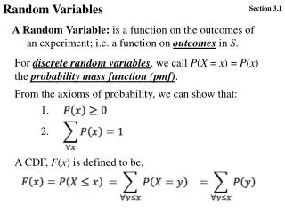
Discrete random variables • Discrete random variables have a pmf (probability mass function), PP(X = a) = P(a) • Example: Coin flip X = 0 if heads X = 1 if tails • What is the pmf of thisrandom variable? Tim Marks, Dept. of Computer Science and Engineering
Discrete random variables • Discrete random variables have a pmf (probability mass function), PP(X = a) = P(a) • Example: Die roll X {1, 2, 3, 4, 5, 6} • What is the pmf of thisrandom variable? Tim Marks, Dept. of Computer Science and Engineering
p(x) 0.5 x 0 1 2 Continuous random variables • Continuous random variables have a pdf (probability density function), p • Example: Uniform distribution p(1.3) = ? p(2.4) = ? What is the probability that X = 1.3 exactly: P(X = 1.3) = ? Probability corresponds to area under the pdf. P(1 < X < 1.5) = ? Tim Marks, Dept. of Computer Science and Engineering
p(h) p(h) p(h) h h h Continuous random variables • What is the total area under any pdf ? • Example continuous random variable: Human heights Tim Marks, Dept. of Computer Science and Engineering
Random variables • How much change do you have on you? • Asking a person (chosen at random) that question can be thought of as sampling from a random variable. • Is the random variable “Amount of change people carry” discrete or continuous? Tim Marks, Dept. of Computer Science and Engineering
Random variables: Mean & Variance • These formulas can be used to find the mean and variance of a random variable when its true probability distribution is known. Definition Discrete r.v. Continuous r.v. Mean Variance Var(X) Tim Marks, Dept. of Computer Science and Engineering
An important type of random variable Tim Marks, Dept. of Computer Science and Engineering
The Gaussian distribution X ~ N(, 2) Tim Marks, Dept. of Computer Science and Engineering
Estimating the Mean & Variance • After sampling from a random variable n times, these formulas can be used to estimate the mean and variance of the random variable. • Samples x1, x2, x3, …, xn Estimated mean: maximum likelihood estimate Estimated variance: unbiased estimate Tim Marks, Dept. of Computer Science and Engineering
Finding mean, variance in Matlab • Samples • Mean>> m = (1/n)*sum(x) • Variance Method 1: >> v = (1/n)*(x-m)*(x-m)’ Method 2:>> z = x-m >> v = (1/n)*z*z’ Tim Marks, Dept. of Computer Science and Engineering
Example continuous random variable • People’s heights (made up) • Gaussian = 67 , 2 = 20 • What if you wentto a planet whereheights wereGaussian with = 75 , 2 = 5 • How would they be different from us? Tim Marks, Dept. of Computer Science and Engineering
Example continuous random variable • Time people woke up this morning • Gaussian = 9 , 2 = 1 Tim Marks, Dept. of Computer Science and Engineering
Let’s collect some samples and graph them: y (wake-up times) x (heights) Random vectors • An n-dimensional random vector consists of n random variables all associated with the same probability space. • Each outcome dictates the value of every random variable. • Example 2-D random vector: where X is random variable of human heights Y is random variable of wake-up times • Sample n times from V. Tim Marks, Dept. of Computer Science and Engineering
Random Vectors • The probability distribution of the random vector P(V) is P(X, Y) , the joint probability distribution of the random variables X and Y. • What will the graph of samples from V look like? • Find m,the mean of V • (Mean of X is 67) • (Mean of Y is 10) Tim Marks, Dept. of Computer Science and Engineering
Mean of a random vector • Estimating the mean of a random vector • n samples from V Mean • To estimate mean of V in Matlab >> (1/n)*sum(v,2) Tim Marks, Dept. of Computer Science and Engineering
Random vector • Example 2-D random vector: where X is random variable of human heights Y is random variable of human weights • Sample n times from V • What will graph look like? Tim Marks, Dept. of Computer Science and Engineering
Covariance of two random variables • Height and wake-up time are uncorrelated, but height and weight are correlated. • Covariance Cov(X, Y) = 0 for X = height, Y = wake-up times Cov(X, Y) > 0 for X = height, Y = weight • Definition: If Cov(X, Y) < 0 for two random variables X, Y , what would a scatterplot of samples from X, Y look like? Tim Marks, Dept. of Computer Science and Engineering
Estimating covariance from samples • Sample n times: maximum likelihood estimate unbiased estimate • Cov(X, X) = ? Var(X) • How are Cov(X, Y) and Cov(Y, X) related? Cov(X, Y) = Cov(Y, X) Tim Marks, Dept. of Computer Science and Engineering
Estimating covariance in Matlab • Samples – Meansmx m_xmy m_y • Covariance Method 1: >> v = (1/n)*(x-m_x)*(y-m_y)’ Method 2:>> w = x-m_x>> z = y-m_y>> v = (1/n)*w*z’ Tim Marks, Dept. of Computer Science and Engineering
Covariance matrix of a D-dimensional random vector • In 2 dimensions • In D dimensions • When is a covariance matrix symmetric? A. always, B. sometimes, or C. never Tim Marks, Dept. of Computer Science and Engineering
Example covariance matrix • People’s heights (made up) X ~ N(67, 20) • Time people woke up this morning Y ~ N(9, 1) • What is the covariance matrix of ? Tim Marks, Dept. of Computer Science and Engineering
Estimating the covariance matrix from samples (including Matlab code) • Sample n times and find mean of samples • Find the covariance matrix >> m = (1/n)*sum(v,2)>> z = v - repmat(m,1,n)>> v = (1/n)*z*z’ Tim Marks, Dept. of Computer Science and Engineering
Gaussian distribution in D dimensions • 1-dimensional Gaussian is completely determined by its mean, , and variance, 2 : • D-dimensional Gaussian is completely determined by its mean, , and covariance matrix, : X ~ N(, 2) X ~ N(,) What happens when D = 1 in the Gaussian formula? Tim Marks, Dept. of Computer Science and Engineering

