Random Variables
Random Variables. 7.1. Random Variables. What you’ll learn What is a Random Variable? Discrete vs Continuous How to construct a valid probability distribution Using the information in a probability distribution to answer probability questions. Random Variable.

Random Variables
E N D
Presentation Transcript
Random Variables 7.1
Random Variables • What you’ll learn • What is a Random Variable? • Discrete vs Continuous • How to construct a valid probability distribution • Using the information in a probability distribution to answer probability questions
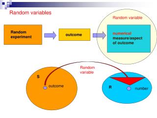
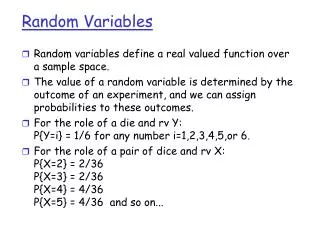
Random Variable • A Random Variable is a variable whose value is numerical outcome of a random phenomenon. • A Random phenomenon has outcomes that we cannot predict, but in the long run has a regular distribution. • Random Variables are either classified as Discrete or Continuous
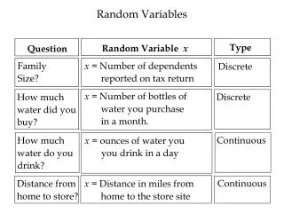
Discrete vs Continuous • Discrete RV: a discrete rv is a variable whose outcomes have a “countable” number of outcomes. • In other words, the outcomes can only take on a finite number of possibilities • Examples: • Dice: If you roll a six-sided die, the possibilities are 1,2,3,4,5, or 6. • Number of A’s, B’s, C’s, D’s and F’s in a classroom
Continuous Random Variable • Continuous: • A continuous variable is a variable that takes on all values within a specified interval • For Example: • Height: only the precision of the measurement instrument dictates the number of decimal places • Weight: again instrument precision • Time: another continuous random variable
Describing a Continuous RV • We describe a Continuous RV using a density curve. • We can calculate probabilities for any given interval by finding the area under the density curve. • These curves can be familiar geometric shapes, such as rectangles (if our distribution is uniform) • A Normal distribution is a Continuous RV • We will concentrate most of our time on discrete distributions, since we have already learned how to calculate probabilities in a normal distribution.
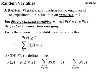
Discrete Probability Distributions • A discrete random variable has a countable number of outcomes. • The probability distribution for a discrete rv lists each of these outcomes and the probability for each outcome
Discrete RV Probability Distribution • Requirements for a VALID probability distribution • Each individual probability must be a number between 0 and 1 • The sum of all the probabilities must equal 1
Discrete Probability Distribution Example • Consider for a moment a large statistics class. • Over the years we know that the distribution of grades has been 15% each of A’s and D’s, 30% each of B’s and C’s and 10% F’s. • Consider choosing a student at random from this class.
Creating a Probability Distn • We can find the probability of the chosen student’s grade by creating the distribution. • Consider the student’s grade on a 4-point scale. A=4, B=3, ect.
Verify the distribution is valid • All probabilities are between 0 and 1 • Sum of the probabilities = 1 • .10 + .15 + .30 + .30 +.15 = 1 • Since both conditions have been met, this is a valid probability distribution
Now let’s use the distribution to find some probabilities • Find the probability that the student got a B in the class • P(X=3) = 0.30 = 30% • We can read this directly from the table
Find the probability that the student got a C or better. • P(x≥ 2) = P(x=2) + P(x=3) + P(x=4) • = .30 + .30 + .15 = .75 = 75% • To find this probability we find each individual probability and find the sum.
Find the probability that the student got less than a B • P(x< 3) = P(x=2) + P(x=1) + P(x=0) • = .30 + .15 + .10 = .55 = 55% • Notice that since we want strictly less than 3, we only find the sum from 2 down.
Inequality Signs • Let’s recall what signs to use when we are looking for inequalities: • Less than < • At Most ≤ • Greater than > • At least ≥ • Remember if the equal sign is included, we include the probability at the endpoint. • If a strict inequality, we do not include the probability at the end point.
Finding the Mean and Standard Deviation • Consider: • As the head of inventory for Knowway computer company, you were thrilled that you had managed to ship 2 computers to your biggest client the day the order arrived. You are horrified, though, to find out that someone restocked refurbished computers in with the new computers in your storeroom. The shipped computers were selected randomly from the 15 computers in stock, but 4 of those were actually refurbished. • If your client gets 2 new computers, things are fine. If the client gets a refurbished computer, it will be sent back at your expense--$100—and you can replace it. However, if both computers are refurbished, the client will cancel the order this month and you’ll lose $1000. What’s the expected value and the standard deviation of your loss?
Mean and Standard Deviation • The first thing we need to do is find the probability distribution for the situation. • Let’s define our random variable as the amount of loss that occurs for the company. • The values that X can take are • 0 100 1000 (2N) (1N/1R ) (2R)
We will use a tree diagram to represent the stages in the event. In order to keep the “tree” manageable, we will define each stage as simply as we can. i.e.—”success” or “not a success” The second stage is to choose the second computer. Again there are two different possibilities The first stage has two possible outcomes New P(New &New) = = .5238 New = .2095 Refurb P(New & Refurb) = Choose a computer = .2095 P(Refurb & New) = New Refurb Refurb P(Refurb & Refurb) = = .0571
Mean and Standard Deviation • Now use these probabilities to create the probability distribution. *Note: the probability of losing 100 happens on 2 branches of the tree We want to know on average, how much of a loss the company would have if this happened month after month.
Mean and Standard Deviation • Now use these probabilities to create the probability distribution. • To find the mean (expected value) of this distribution we can use the following: • Μ(x) = E(x) = ∑X· P(X) • The value of the variable times its probability for each, then find the sum.
Mean and Standard Deviation • So for our distribution • Μ(x) = E(x) = ∑X· P(X) • M(x) = E(x) = 0(.5238) + 100(.4190) + 1000(.0571) = 99.00 • So the average loss for Knowway Computers is $99.00
Mean and Standard Deviation • We can find the standard deviation in much the same way we find the standard deviation for a sample • First, let’s find the variance • σ2= ∑(x-μ)2 ·P(x) • (0 – 99)2 (.5238) + (100-99)2(.4190) + (1000-99)2(.0571) = 51488.0199 Dollars2
Mean and Standard Deviation • So, the variance is 51488.0199 dollars2 • But we need the standard deviation which will bring our units back to dollars • Remember that standard deviation is the square root of the variance so…. • σ = √51488.0199 = $266.91
Mean and Standard Deviation • We can use our calculators to find both the mean and standard deviation of a probability distribution. • Enter the values of the RV in one list • Enter the probabilities for each value into a second list • Use Stat/Calc/1-var statistic (Xlist, Problist) • The mean will be under x-bar • The standard deviation will be sigma


