Random Variables
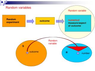
Presentation 6. Random Variables. Random Variables. A random variable assigns a number (or symbol) to each outcome of a random circumstance. Example: Lets call our random variable X! Let X = the number of spades in a random sample of 4 cards from a deck.

Random Variables
E N D
Presentation Transcript
Presentation 6. Random Variables
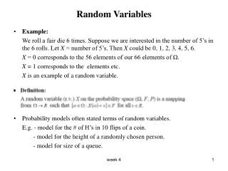
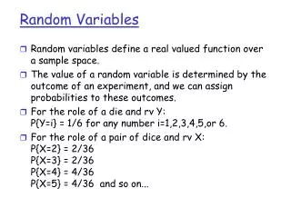
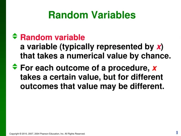
Random Variables • A random variable assigns a number (or symbol) to each outcome of a random circumstance. Example:Lets call our random variable X! • Let X = the number of spades in a random sample of 4 cards from a deck. • Let X = the sum of 2 rolls of a six sided die. • Let X = the number of people with blue eyes in a sample of 10 people. • Let X = the weight of a randomly chosen person.
Two types of Quantitative R. Vs • Discrete Random Variables • Result in a countable set of possibilities (e.g. only integer values.) • Cannot take any possible value in an interval (since there are uncountable many values in an interval). Examples: 1. X = the sum of 2 rolls of a six sided die. Outcomes: 2-12 2. X = number of tosses until the first “head”. Outcomes: 1,2,3,… • Continuous Random Variables • The outcome can be in any interval or collection of intervals. Examples: 1. X = Time spent waiting for the bus. 2. X = the weight of a randomly chosen individual. Outcomes: 120 lbs, 120.00001lbs, 183.12302 lbs,…
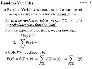
Discrete Random Variables Probability Notation and Distributions • X = the random variable. • k = a number that the discrete r.v. could assume (a possible outcome!) • P(X=k) is the probability that X equals k. • The probability distribution function (PDF) for a discrete random variable is a table or rule that assigns probabilities to the possible outcomes of a random variable X.
Discrete Random Variables Example Assume the probability of a girl is ½. Let X = the number of girls in a family with 3 children. What is the probability distribution of X? Possible Outcomes: 0, 1, 2, or 3 girls. Event: BBB BBG BGB GBB BGG GBG GGB GGG Prob: 1/8 1/8 1/8 1/8 1/8 1/8 1/8 1/8 X: 0 1 1 1 2 2 2 3 PDF of X:
Discrete Random Variables Cumulative Distribution Function • The Cumulative Distribution Function for a random variable X is rule or table that provides the probabilities P(X ≤ k). The term ‘cumulative probability’ refers to the probability that X is less than or equal to a particular value. Example: Number of Girls CDF of X:
Discrete Random Variables Expectations • The expected value of a random variable is the mean value of the variable X in the space of possible outcomes (or population). Also can be interpreted as the mean value from an infinite number of observations of the random variable. It is also denoted with the Greek letter μ. E(X) = μ = So the expected value of the number of girls is E(X)= μ = 0*1/8 + 1*3/8 + 2*3/8 + 3*1/8 = 3/8+6/8+3/8 = 12/8 or 1.5 girls!
Special Case of Discrete Random Variables: Binomial Random Variables Binomial Experiment is defined by the following: • There are n “trials” where n is determined in advance. • There are two possible outcomes on each trial, a “success”, and a “failure”. • The outcomes are independent from one trial to the next. • The probability of a “success” remains the same from one trial to the next and is denoted by p.
Binomial Random Variables • If we have a Binomial experiment with n trials and p probability of success, then X= number of successes (out of n trials), is called a binomial random variable. What is the sample space of X? Example: Drawing 10 cards from a deck with replacement and counting the number of spades. Then, we have the binomial random variable X = ______________________________ sample space of X = ________________
PDF, Expectation, and Standard Deviation of a Binomial Random Variable P(X=k) = E(X) = μ= S.D.(X) = σ = Note: n! = 1x2x…xn, e.g. 3!=1x2x3=6 Example: Number of Girls
Example Binomial: Number of Spades in 10 draws:
Special Case of Continuous Random Variables: Normal Random Variables • In the class of continuous random variables, we are primarily interested in NORMAL random variables. • These are a continuous random variable with a bell-shaped distribution. These normal or bell-shaped variables occur often in nature. Example:Heights of Males are Normally Distributed Probability Density Function for Heights of Males --->
Probabilities with Normal RVs • When we consider Normal Random Variables (or any continuous r.v.), we are interested in the probability that X falls into some INTERVAL. • There are infinitely many normal pdf’s (curves). To fully describe a normal curve, we need the location (mean, μ) and the spread (s.d., σ). • When talking about the population mean and s.d. we use the Greek letters μ and σ, when talking about the sample mean and s.d. we use and s. Example:Suppose X is the height of a randomly chosen college woman. Further suppose that the heights of college women can be described as a normal, with μ = 65inches, and σ = 2.7 inches. We might ask: • What is the proportion of women that are shorter than 62 inches? • What is the probability that X is between 65 and 67 inches?
Graphical Representation of Probabilities P(65<X<67) P(X<62) Note: The total area under the curve is equal to 1!
How to Calculate Probabilities If you want P(X<x) where x equals some value, first compute a z-score! z = (Value – mean)/(Standard Deviation) z = (x-µ)/σ, P(X<x) = P(Z<z) for which we have tables!! Examples: 1.P(X<62) z = (62 – 65)/2.7 = -3/2.7 = -1.11 P(X<62) = P(Z < -1.11), now use Normal Table (Table A.1, page 538 in your text) P(Z< -1.11) = 13.4% 2.P(65<X<67) z1 = (65 – 65)/2.7 = 0, z2 = (67 – 65)/2.7 = 1.11 P(65<X<67) = P(0<Z<1.11) = P(Z<1.11) – P(Z<0) P(Z<1.11) – P(Z<0) = .867 – .5 = .367 or 36.7% 3.P(X>62) = 1-P(X<62) = 1-0.134 = 0.866
Some notes for calculating probabilities • The normal table provides probabilities of the form P(Z<“number”). • For continuous random variables the probability of being less than or less of equal than a number are the same. (e.g. P(Z<2.1) = P(Z 2.1)) • It is always a good idea to draw a normal curve and shade the area corresponding to the probability of interest. • If c, c1, c2 are some numbers, then • P(Z>c) = 1 – P(Z<c) • P(c1<Z<c2) = P(Z<c2) - P(Z<c1) Draw a normal curve and shade the areas corresponding to the above probabilities. Can you see why we have these equalities?
Example: Suppose verbal SAT scores of high-school freshman are normally distributed with a mean of 500 and a standard deviation of 50. • What is the probability of a randomly chosen individual having a score greater than 600? z-score = [600-500]/50 = 2 P(X>600) = P(Z>2) = 1- P(Z 2)= 1-P(Z<2) = 1-.9772 = 0.228 Note that the only difference in the two graphs below is the scale on the tow axes. However, the shaded areas are equal…since the total area under any of this curves is one. P(X>600) P(Z>2) -4 -2 0 2 4
What is the probability of a randomly chosen individual having a score between 400 and 500? We want P(400<X<500). z-score1 = z1 = [400-500]/50 = -2 z-score2 = z2 = [500-500]/50 = 0 P(400<X<500) = P(-2 < Z < 0) = P(Z<0) – P(Z<-2) = .5-.228 = .4772 (from Table) P(-2<Z<0) That is the probability of a randomly chosen student having a score between 400 and 500 is about .48 or 48%.
What is the probability of a randomly chosen individual having a score between 350 and 450? z-score1 = z1 = [350-500]/50 = -3 z-score2 = z2 = [450-500]/50 = -1 P(350<X<450) = P(-3 < Z < -1) = P(Z<-1) – P(Z<-3) = .1587-.0013 = .1574 (from normal Table) P(-3<Z<-1) That is the probability of a randomly chosen student having a score between 350 and 450 is about .16 or 16%.
Approximating binomial distribution probabilities • Suppose X is a binomial distribution with trials n and success probability p. • >10 and >10 (i.e. the expected number of both, successes and failures, in the sample is greater than 10.) • X is approximately a normal random variable with mean m= and standard deviation s=
Normal appr. of binomial variables Let X be a binomial distribution with n=20 and p=0.5. • Check if the approximation rules are satisfied? • What is the mean and the s.d. of X? • Compute P(X≤10) by two ways: • Using minitab to compute P(X≤10) where X is a binomial r.v. with n=20 and p=0.5, we get P(X≤10) =0.5881 • Using normal approximation: for X a normal r.v. with μ=______ and σ=________ we get P(X≤10)=0.5
SummaryDefinitions and theory for binomial rv’s • If X is a r.v. representing the number of successes in n independent, identical trials, with probability of success p remaining constant from trial to trial, then is called a binomial r.v. with parameters n and p. • The cumulative density function (cdf) of X is P(X ≤ k), for all k. • For k integer between 0 and n we have that P(X < k) = P(X ≤ k-1) • Note that is not true for discrete random variables in general!!! Binomial random variables can take only the integer values 0,1,…,n (since is the number of successes out of n). If X is not a binomial variable it might be the case that the possible values of X are 2, 2.5, 3, 3.5 and 4. Then, in this case P(X < 3) = P(X ≤ 2.5). • For a binomial random variable X with n number of trial and p prob. of success μ = E(X) = σ = • So…for binomial random variables you do not need to use the general formula for the expected value of discrete r.v.’s!
SummaryDefinitions and theory for Normal r.v’s. • Knowing μ and σ, specifies the particular normal distribution out of the class of all normal distributions. (Similarly, knowing n and p, specifies a particular binomial distribution.) • The pdf of any normal r.v X, also called normal curve, is symmetric, bell shaped and centered at the mean, μ. • The standard normal random variable has mean 0 and standard deviation 1. We denote it with Z. • We have the tables for all the probabilities of the form P(Z ≤ z). So, for any normal r.v X, with mean μ and standard deviation σ, we can obtain any probabilities of interest using the following “standardization theorem’. If X has a normal distribution with mean μ, and standard deviation σ, then {(X- μ)/ σ } has a normal distribution with mean 0, and standard deviation 1, P(X ≤ x) = P [(X- μ)/ σ ≤ (x- μ)/ σ] = P[Z ≤ (x- μ)/ σ] = P(Z ≤ z), Where z = (x- μ)/ σ, is called the z-score of x.
SummaryFinding Probabilities of X • First find the z-score of x (or x’s if more than one) to be able to use the tables. • Think what is the area under the curve that corresponds to this probability. • Figure out how you can get this probability using probabilities rules and values form the tables. • Have in mind that the normal curve is symmetric and that the total area under the curve is equal to 1. • The empirical rule for the standard deviation on page 44, is valid for all bell-shaped distributions (μ ± σ, μ ± 2σ, μ ± 3σ, approximate intervals), but it is EXACTLY RIGHT in the case of normal distribution. i.e. P(-1<Z<1) = _______, P(-2<Z<2) = _______, P(-3<Z<3) = ________ • How can we find percentiles? i.e. for a normal r.v. X with mean μ and standard deviation σ , how can we find x (a value of X), such that P( X ≤ x) = α, where α is α known probability. e.g. if α = 95% (we want to find the 95th percentile of X). First we get the α-th percentile for Z, P(Z≤ z) = 0.95, then z = 1.64. and we get x using x= σ z + μ

