Download
1 / 39
420 likes | 577 Vues
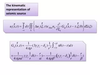
The kinematic representation of seismic source. The double-couple solution. double-couple solution in an infinite, homogeneous isotropic medium. NF. IT. FF. Radiation Pattern. moment rate function. Far Field representation. Far Field representation homogeneous, isotropic, elastic medium.

E N D
The double-couple solution double-couple solution in an infinite, homogeneous isotropic medium. NF IT FF Radiation Pattern moment rate function
Far Field representationhomogeneous, isotropic, elastic medium Neglecting all terms that attenuate with distance more rapidly than 1/r
Far Field representationhomogeneous, isotropic, elastic medium If the receiver is far enough away with respect to the linear dimension of fault L, we can assume that the distance and the direction cosines are approximately constant, independent of x. Thus, the constant or slowly variable factors can be moved outside the integral
Far Field Displacement pulse Final slip in following slides
Fraunhofer Approximation The error in this approximation is
DISPLACEMENT FOURIER SPECTRUM Acceleration The ground displacement Fourier spectrum is nearly flat at the origin displacement Corner frequency
Far Field representationinhomogeneous, isotropic, elastic medium If the receiver is far enough away with respect to the linear dimension of fault L, we can assume that the distance and the direction cosines are approximately constant, independent of x. Thus, the constant or slowly variable factors can be moved outside the integral
Aki – Richards, 2002, p.499 Unilateral Rupture propagation Source time function Y is the angle between the direction of rupture propagation and the direction of the receiver The integrand of this equation ranges between and The pulse is proportional to a moving average of taken over a time interval of duration
Unilateral Rupture propagation • Taking Fourier Transform The term sin(X)/X expresses the effect of fault finiteness on the amplitude spectrum. At high frequency this term is proportional to w-1. The smoothing effect is weakest in the direction of propagation (y=0) and strongest in the opposite direction (y=p). Thus, we observe more high-frequency in the direction of rupture propagation: that is DIRECTIVITY
Tr = rise time t The effect of finite rise time t < tr = x / vr Tr< t < T + tr t > T + tr The effect of finite rise time introduces an additional smoothing of the waveform: for high frequency it attenuates the spectrum proportional to w-1. Together with the effect of the term sin(X)/X, the spectrum decays astow-2.
Some properties At w= 0 it is proportional to WLDmax, which is the seismic moment At frequency larger than the characteristic frequency given by 1/T or 1/L(1/v – cos(Y)/c) the spectrum attenuates as w-2 If the effect of finite width is taken into account, we have a high frequency spectral decay proportional to as w-3
A brief note on earthquake dynamic Slip, Slip velocity & Traction evolution
A brief note on earthquake dynamic The Slip Weakening mechanism
A case study: The 1997 Colfiorito Earthquake Normal faulting earthquakes Multiple main shocks of similar size Moderate magnitudes
Peak ground motionattenuationa) Colfiorito eventunilateral NW ruptureb) Sellano eventnearly unilateralSE propagation
Colfiorito earthquake • Some spectra
Comparison between predicted and observed PGA Colfiorito earthquake
Comparison between predicted and observed data with empirical regression law
The 2007 Niigata-ken Chuetsu-oki earthquake KKNPP is the nuclear power plant
Waveform inversion to infer seismic source Seismic source models obtained by inverting seismograms and GPS displacements
Ground Motion Prediction through the inferred model
Spectral models Omega cube model Omega square model
Computing earthquake magnitude M = log (A/T) + F(h,R) + C A – amplitude T – dominant period F – correction for depth & distance C – regional scale factor
Seismic Moment & Magnitude From seismic moment we can compute an equivalent magnitude called the moment magnitude
Scaling of final slip with fault length Wells & Coppersmith 1994
STRESS DROP SCALING is a factor depending on fault’s shape For a circular fault with radius R
Stress and Radiated Energy Strain energy release Seismic efficiency Apparent stress
A slip weakening model Energy loss