Computational Fluid Dynamics - Fall 2007
Computational Fluid Dynamics - Fall 2007. The syllabus CFD references (Text books and papers) Course Tools Course Web Site: http://twister.ou.edu/CFD2007 http://learn.ou.edu Computing Facilities available to the class (account info will be provided)

Computational Fluid Dynamics - Fall 2007
E N D
Presentation Transcript
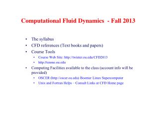
Computational Fluid Dynamics - Fall 2007 • The syllabus • CFD references (Text books and papers) • Course Tools • Course Web Site: http://twister.ou.edu/CFD2007 • http://learn.ou.edu • Computing Facilities available to the class (account info will be provided) • OSCER (http://oscer.ou.edu) Topdawg Linux Supercomputer • Unix and Fortran Helps – Consult Links at CFD Home page
Introduction – Principle of Fluid Motion • Mass Conservation • Conservation of air mass • Conservation for other material quantities (e.g., CO2 or water vapor in atmosphere) • Newton’s Second of Law (equations of motion) • Energy Conservation (e.g., temperature equation) • Equation of State for Idealized Gas • Other equations These laws are expressed in terms of mathematical equations, usually as partial differential equations. Most important equations – the Navier-Stokes equations
Approaches for Understanding Fluid Motion • Traditional Approaches • Theoretical – find analytical solutions • Experimental – collect data from laboratory or field experiments • Newer Approach • Computational - CFD emerged as the primary tool for engineering design, environmental modeling, weather prediction, oil reservoir simulation and prediction, nuclear weapon testing, among many others, thanks to the advent of digital computers
Theoretical FD • Science for finding usually analytical solutions of governing equations in different categories and studying the associated approximations / assumptions; h = d/2,
Experimental FD • Understanding fluid behavior using laboratory models and experiments. Important for validating theoretical solutions. • E.g., Water tanks, wind tunnels
Computational FD • A science of finding numerical solutions of governing equations, using high-speed digital computers
Why Computational Fluid Dynamics? • Analytical solutions exist only for a handful of typically simple problems • Much more flexible – easy change of configurations, parameters • Can control numerical experiments and perform sensitivity studies, for both simple and complex systems or problems • Can study something that is not directly observable (e.g., black holes of the universe or the future climate) because of the spatial and/or temporal scale of the problem. • Computer solutions provide a more complete sets of data in time and space than observations of both real and laboratory phenomena
Why Computational Fluid Dynamics? - Continued • We can perform realistic experiments on phenomena that are not possible to reproduce in reality, e.g., the weatherand climate • Much cheaper than laboratory experiments (e.g., crash test of vehicles, experimental launches of spacecrafts) • May be much more environment friendly (testing of nuclear arsenals) • We can now use computers to DISCOVER new things (drugs, sub‑atomic particles, storm dynamics) much more quickly • Computer models can predict, e.g., weather.
An Example Case for CFD – Thunderstorm Outflow/Density Current Simulation
Positive Internal Shear g=1 Negative Internal Shear g=-1
T=12 Positive Internal Shear g=1 Negative Internal Shear g=-1 No Significant Circulation Induced by Cold Pool
Simulation of an Convective Squall Line in Atmosphere Infrared Imagery Showing Squall Line at 12 UTC January 23, 1999. ARPS 48 h Forecast at 6 km Resolution Shown are the Composite Reflectivity and Mean Sea-level Pressure.
10 minute time intervals Movie of WRF 2 km forecast v.s. observations during Spring 2007 Forecast Experiment (Xue et al. 2007)
Difficulties with CFD • Typical equations of CFD are partial differential equations (PDE) that requires high spatial and temporary resolutions to represent the originally continuous systems such as the ocean and atmosphere • Most physically important problems are highly nonlinear ‑ true solution to the problem is often unknown therefore the correctness of the solution hard to ascertain – need careful validation (against theoretical understanding and limited measurement data)! • It is often impossible to represent all relevant scales in a given problem ‑ there is strong coupling between scales in atmospheric flows and most CFD problems. ENERGY TRANSFERS among scales.
Difficulties with CFD • The initial conditions of given problems often contain significant uncertainty – such as that of the atmosphere – because they can’t be measured with 100% accuracy • We often have to impose nonphysical boundary conditions. • We often have to parameterize processes which are not well understood (e.g., rain formation, chemical reactions, turbulence). • Often a numerical experiment raises more questions than providing answers!!
Positive Outlook • New numerical schemes / algorithms • Bigger and faster computers (Petascale Computing Systems to be built – first at NCSA) • Faster networks • Better desktop computers • Better programming tools and environment • Better visualization tools • Better understanding of dynamics / predictabilities • etc.