Computational Fluid Dynamics Course Notes
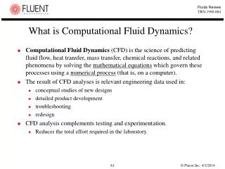
Learn the basics of Computational Fluid Dynamics (CFD) and an introduction to CFX software. Understand the physics, equations, solution methods, grid creation, data visualization, and solution techniques.


Computational Fluid Dynamics Course Notes
E N D
Presentation Transcript
Computational Fluid Dynamics Course Notes Dr PK Dyson Sep 2004
CFD Overview and Introduction to CFX
Introduction What do you want to know? What do you need to define? What’s the physics?
Solution of the Equations • Equations are solved numerically, at a series of discrete points in the flow domain. • 5 variables at 100,000 points implies what ….? • Results can be viewed graphically and processed to provide numerical outputs. For most packages, the data stream is: Geometry >> Mesh creation >> Fluid definition >> Problem definition >> Solution >> Viewing of Results CAD (usually) Mesh Generator Pre-processor Solver Post-processor
ANSYS – CFX Overview (1) Start > University Software > ANSYS > ANSYS 10 This starts the ANSYS Workbench environment from which the various individual components are launched. ANSYS Workbench (*.wbdb file) CAD Import Mesh Control Parameters Geometry DesignModeller (*.agdb file) CFX-Mesh (*.cmdb file) Geometry file (*.gtm)
ANSYS – CFX Overview (2) Geometry file (*.gtm) Problem type Solution control CFX-Pre Case file (*.cfx) Boundary conditions Session file (*.ses) holds record of commands entered during session Fluid properties Journal file (*.jou) holds record of commands for particular database Definition file (*.def)
ANSYS – CFX Overview (3) Definition file (*.def) Solver Output file (*.out) Results file (*.res) (numerical data in text file) CFX-Post Forces Velocities Streamlines Numerical output (via calculator and export) Pressures Turbulence See Help:- from Advanced CFX Panel: Help > Master Contents ANSYS CFX, Release 10.0: Installation and Overview > Overview of ANSYS CFX > ANSYS CFX File types
File Management • Create a “MyCFX” folder on the local hard drive and put each job in a different sub-folder. • Do not leave spaces in folder or file names anywhere in the path to your working folder. • Work from the local hard drive or pen drive (not across the Network from your U: drive) • At the end of the session, drag and drop your entire working folder to your pen drive. • WARNING: Always keep files on you own independent storage media – the hard drives are cleaned each night.
Contact with ANSYS-CFX Staff IMPORTANT NOTE If you encounter problems with CFX, then by all means visit the CFX Community pages (address is on the Resources Sheet), but do not contact ANSYS-CFX Staff until you have first discussed your problems with UoP staff. Contact with ANSYS-CFX should normally be through UoP Staff.
General Principles - Revision Mass Continuity u2 u1 For steady flow Momentum net force acting on fluid = rate of change of momentum = change of rate of mom’m flow = how?
Mass Continuity Equation (1) mass-velocity = u y y,v x z,w v x,u Net rate of outflow of mass = rate of depletion of mass in control volume
Mass Continuity Equation (2) Substantial derivative For incompressible flow, this becomes:
Momentum Equation (1) Force on Control Volume = Rate of Change of Momentum Velocity Changes across Control Volume u y x v
Momentum Equation (2) Forces Acting in x-Direction on Control Volume y x
Momentum Equation (3) Rate of Change of Momentum in x-direction = 0 for steady flow (from continuity)
Momentum Equation (4) Net force in x-direction
The Navier-Stokes Equations For: • steady state • 2-dimensional • incompressible
Navier-Stokes - Summation Convention Taking u = u1 v = u2 w = u3 (separate equation for each of i = 1 to 3 • where • 1, 2, 3 represent x, y, z directions • a subcripted comma and index represents a derivitive • repeated subscript means set it to 1, 2, 3 in turn and sum resulting variables (so what does uj,j = 0 mean?)
The Energy Equation Internal generation u y x v Convection with mass transfer Conduction by temperature gradient
Analytical Example - Couette Flow Moving Plate - vel = us s Infinitely long y Stationary plate x
Solutions to the Equations The set of equations for incompressible, viscous, 2D steady flow is: Unknowns are u, v, P which are to be solved in terms of x and y - i.e. across flow domain. Solutions are typically plots of velocity vectors, streamlines, pressure contours (and temperature contours if energy equation is added). These may be processed to produce such data as forces (eg lift and drag on a foil) or pressure loss in pipes and fittings.
Computational Grid Since analytical solution is available only in simplest of cases, numerical techniques are required; thus a grid across flow domain needs to be defined Unknowns are determined at each grid point Concept may be extended into time domain: t x y
Typical Grid Notation i+1, j+1 i-1, j+1 i, j+1 i, j i+1, j i-1, j i, j-1 i+1, j-1 i-1, j-1
Solution Techniques • Broadly speaking, one of three techniques is adopted for the solution of the governing equations: • finite difference, in which the differential terms are discretised for each element • finite volume, in which the governing equations are integrated around the mesh elements • finite element, in which variation of variables within elements is approximated by a function, and a residual (or error term) is minimised. • The first of these is perhaps the easiest conceptually, and thus we will use this to outline a typical solution procedure. • CFX uses the finite volume method.
Differencing Formulae (1) u ui+1 ui i i+1 x Taylor Expansion (second order central difference)
Differencing Formulae (2) Adding the Taylor Series equations: Thus, if we take, say, the x direction N-S equation (steady for simplicity):
The Equation Set If we set up this set of equations at each of n interior points in the domain, and we know the boundary conditions (b) at the exterior points …. b b b b b b b b b b b b …. then we will form 3n simultaneous equations in 3n unknowns. Unfortunately, these are non-linear, so an iterative approach is usually employed - eg. guess u, v for the domain and insert as ui,j, vi,j in previous set of equations insert revised values of ui,j,vi,j solve equations for u, v, P check convergence
The Pressure Correction Approach Semi-Implicit Method for Pressure Linked Equations - SIMPLE !!!! Guess a pressure field Solve N-S equations (not continuity) for u,v, given these guessed pressures Solution process may be iterative or time marching Use modified continuity equation to calculate a pressure correction Do u, v values satisfy continuity? (convergence criterion) N Y Finish
Boundary Conditions (1) • Boundaries must be defined, but care must be taken not to: • under-define boundaries (insufficient data for solution) • over-define boundaries (creating a physically impossible situation) • eg. With parameters defined on boundaries as follows ….. wall u=0,v=0 u=value v=0 P=value u=value v=0 P=value u=0,v=0 wall ……… model is over-defined since velocity and pressure are stipulated at inlet and outlet. Values may thus not satisfy the continuity and momentum equations.
Boundary Conditions (2) Boundaries defined will depend on nature of equations to be solved (steady / unsteady, incompressible / compressible, inviscid / viscous) For example, for steady, incompressible, viscous flow, solved by pressure correction method, boundaries conditions may be: v = 0 P= value P= value
Grids (1) Structured Mesh usually comprising quadrilateral elements Physical Space eg. circular duct Computational Space
Grids (2) Aerofoil Section (Example of structured mesh, refined in critical regions)
Grids (3) Unstructured Mesh usually based on triangular pyramids (eg CFX 5) • Important Modelling Considerations • Grid refinement in critical areas • Grid independent solution - checks required • Computationally economic model • coarse grid in non-critical areas • make use of symmetry and periodic boundary conditions • use 2-D and axi-symmetric models where possible
vel at a point Turbulence u’ time
Introduction to Turbulence Modelling Laminar Flow Momentum diffusion by viscosity Turbulent Flow Additional momentum diffusion due to turbulence Concept of turbulent (or eddy) viscosity, t • t is not a fluid property, but depends on level of turbulence in flow • concept leads to mathematical models to deal with turbulence; each model is an approximation to what is really happening • one popular model (k-epsilon model) introduces two further unknowns:
Turbulence Modelling – the Maths Think of u,v,w and p as comprising of two parts: ensemble average values and turbulent fluctuations. Superscript bar denotes the ensemble average or the mean value. Dash denotes the fluctuating part. Turbulence fluctuations usually have small length and time scales compared to the mean flow. Substituting this decomposition to the Navier-Stokes equations and taking the ensemble average, we now get
Turbulence Closure • Equations (also called Reynolds equations) for ensemble average values are identical to the Navier-Stokes equation except for the cross-products of the fluctuation terms. • Since these terms have similar functions as viscous stresses, they are called ‘turbulent stresses’ or Reynolds stresses. • To properly close the system, we have to define the behaviour for turbulence cross-product terms. • This is where many different types and levels of turbulence modelling come in. • At the highest level, transport equations can be set up for each of these terms. This will increase the number of equations to solve by six. Turbulence models based on this approach are called Reynolds stress equation model (RSM) or the second-order closure model. • A commonly used turbulence model in engineering differs from this approach by reducing the number of extra equations to only two and is known by the name k-εmodel.
k-ε Model - Theory In this model, the Reynolds stresses are linked to the mean flow; i.e. where μt is the coefficient for turbulent viscosity and is linked to the turbulent kinetic energy k and dissipation ε. The two extra equations that are needed for the closure are the transport equations for k and ε.
k-ε Model – Theory (continued) Where The (empirical) constants in the k-ε model are usually:
k- Turbulence Model - Summary • requires two further equations, similar to Navier-Stokes equations for k and • thus requires • inlet values for k and • initial guesses for k and • estimates for these may be obtained from equations such as the following, available in the literature • sensitivity to inlet turbulence quantities should be checked, and may point to the need for experimentally derived values for use in the CFD model.
CFD Health Warning ! • We have barely scratched the surface of the theory of CFD. A few of the possible areas for further fruitful reading are: • nature of the equations under different conditions - hyperbolic, parabolic, elliptic. • transient problems • choice of boundary and initial conditions • coupling between momentum and energy equations (especially in buoyancy driven flows) • supersonic flows and shock capture • turbulence modelling - what alternative models are available? • wall boundary conditions (log law of the wall) • Treat CFD with respect - a little knowledge is a dangerous thing !
Exercise 1 • Create folder MyCFX and a sub-folder Tutorial_1 • Start ANSYS CFX 10.0. • In the Launcher, set the Working Directory to the sub-folder you have just created and then go to ANSYS > Workbench 10.0. • In the Start panel that now opens, click Empty Project (under “New”) • Go to Help > ANSYS DesignModeller Help. In the Contents panel, expand the CFX-Mesh Help tree and click Tutorials. Click “Click here”. • Work through Tutorial 1: Static Mixer. • This will take you through: • Geometry creation using DesignModeller • Mesh generation using CFX-Mesh • At the end of this tutorial, under the paragraph “If you want to continue by working through the ANSYS CFX example …”, follow steps 1, 2 and 3 to open the mesh in CFX-Pre. • Now click Help > Tutorials which will take you into the CFX (Fluid Modelling) Tutorials (as opposed to the DesignModeller/CFX-Mesh (Solid Modelling) Tutorial you have just been working through) and click “Flow in a Static Mixer”.
Exercise 1 (continued) • Continue with this tutorial, but note the instructions in para 4 at the end of the DesignModeller Tutorial:- • “… missing out the instructions in the section “Creating a New Simulation”. Note that you do not need to copy the sample file StaticMixerMesh.gtm to your working directory if you have just created the mesh in CFX-Mesh, since you will want to use your new mesh and not the one supplied with ANSYS CFX. For the “Importing a Mesh” section, the only action that you need to carry out is to select Assembly from the Select Mesh drop-down list, as the mesh is loaded automatically when you start ANSYS CFX in the manner described above. “ • This will take you through: • Problem Definition using CFX-Pre • Solution using CFX Solver Manager • Viewing of results using CFX-Post
Now make sure you understand ….. • What’s the difference between • Sketching mode and modelling mode • DesignModeller and CFX-Mesh • Surface Mesh and Volume Mesh … and now consolidate what you’ve done by looking through this example …. In ANSYS Workbench go to Help > ANSYS Workbench Help and in the Contents Tree go to DesignModeller Help >Welcome to the DesignModeller 10.0 Help > Process for Creating a Model Read through the pages and run the video sequences to remind yourself of the process of creating a geometry.
Exercise 2 • Work through Tutorial 2, Static Mixer(Refined Mesh) which will show you: • more about the mesh generation process • modifying geometry • use of CFX Command Language (CCL) to avoid too many repetitive keystrokes. • As before you will need to start in the DesignModeller/CFX-Mesh (Solid Modelling) Tutorial and switch to the CFX (Fluid Modelling) Tutorial.
Exercise 3 • Refine the mesh even further in the outlet region of the mixer by inserting a mesh control as follows. • Re-open StaticMixer in CFX-Mesh • Right click Control > InsertPoint Spacing • Click Point Spacing 1 in Detail View and change the settings to: Length scale 0.1 m, Radius of Influence 0.5 m, Expansion Factor 1.2 • Right click Point Spacing > Insert Line Control • Click Line Control 1 • In Detail View, for point 1 click Apply, and accept coordinates as 0,0,0. Repeat for point 2 and make coordinates 0,0,-2. Click in the box next to spacing, then click Point Spacing 1 in Tree View & click Apply. • Right click Body 1 > Suppress and observe position of Line Control. Unsuppress Body 1. • Generate the surface mesh as before and note the difference around the exit. • Generate Volume Mesh, apply the physics (use import CCL in Pre), Run Solver and view results.
Finding Out More – The Help Pages Help onANSYS Workbench, DesignModeller and CFX-Mesh is available on the Workbench Help button and the subsequent Folder Tree • Help on CFX Pre, Solver and Post is accessed from the Advanced CFD panels (-Pre, -Solver, -Post) by clicking: • Help >Master contents Now use the Help pages to answer the following questions.