WEMBA B, Causal Research, Conjoint Analysis Entitle Insurance

1. WEMBA B, Causal Research,Conjoint AnalysisEntitle Insurance Market IntelligenceJulie Edell Britton Session 7 September 25, 2009

2. Today’s Agenda • Announcements • WEMBA A • Causal Research – Experiments • Pre-experimental Designs • True Experiments • Factorial Designs and Interaction Effects • Conjoint Analysis

3. Announcements • Submit IBM Global Mobile Computing slides by 10 pm tonight!

4. Become a Duke MBA WEMBA (A): School Choice Model Values Perceptions Individual Differences & Constraints • Assumes that behavior is driven by differences in: • Values (Importance of key attributes) • Perceptions (Duke and Competition on key attributes) • Individual Differences & Constraints (travel, cost, etc.) 4

5. The Funnel Attend Information Session Do not attend Information Session Do not apply Do not apply Apply Selected Out Admitted Opt Out Matriculate

6. The Analysis Approach • Sample groups that differ in behavior • Compare the groups on relevant dimensions: • Perceptions • Values • Individual Difference & Constraints • Infer that any difference found between groups are partly responsible for differences in behavior 6

7. WEMBA B • What factors drive application? • Perception of Duke – Perception of Comp • Individual difference measures (demos, % paid by company, etc.) • Conditional on applying, what drives acceptance? • How do info sessions alter perceptions of Duke? • Who should Nagy target, and how can he reach target? • What perceptions might Nagy try to alter with info sessions? 7

8. Today’s Agenda • Announcements • WEMBA A • Causal Research – Experiments • Pre-experimental Designs • True Experiments • Entitle Case • Factorial Designs and Interaction Effects • Conjoint Analysis

9. Causal Research - Validity • The strength of our conclusions • i.e., Is what we conclude from our experiment correct? • Threats to Validity • History: an event occurring around same time as treatment that has nothing to do with treatment • Maturation: people change pre to post • Testing: pretest causes change in response • Instrumentation: measures changed meaning • Statistical Regression: Original measure was due to a random peak or valley 9

10. Online Investor Performance • X = brick and mortar brokerage customer moves online to trade in 1999 • O = Annualized turnover • 1998 – 40% annualized turnover • 2000 – 100% annualized turnover • Did going online cause people to trade more actively? • Threats with one-group pre-post? 10

11. Quasi-Experimental Designs: Interrupted Time Series • Same as one-group pretest posttest, but observations at many points in time before and after key treatment for same people: • EG O1 O2 O3 X O4 O5 O6 • Extra time periods help control for history, maturation, testing. “Quasi-experiment” 11

12. Online Investor Performance 12

13. Portfolio Turnover 13

14. 2 Groups: Unmatched Control Group(Effect of Prior Knowledge on Search) • Hypothesis: People with little knowledge about cars search less online • 100 Durham residents who are in the market for a car • Experimental Group X1 (Auto Shop Course) O1 (6 hrs online) • --------------------------------------------------------- • Control Group X2 (Electronics Course) O2 (3 hrs online) 14 14

15. 2 Groups: Matched Control Group (True Experiment) Experimental Group R X1 (Auto Shop Course) O1 (6 hrs) --------------------------------------------------------- Control Group R X2 (Electronics Course) O2 (3 hrs) Control for Selection Threat Key Point: For causal research, chance (not respondent) must determine respondent assignment to condition. 15 15

16. Breckenridge Brewery Ads • Breckenridge Brewery wants to assess the efficacy of TV ad spots for its new amber ale. • Time 1 (O1): Duke undergrads are brought to the lab and asked to rate their frequency of buying a series of brands in various categories over the past week. The list includes Breckenridge Amber Ale. Mean = 0.2 packs per week. • Time 2 (X): Two weeks of ads for Breckenridge Ale. • Time 3 (O2): Same Duke undergrads brought back to lab to rate frequency of buying same set of brands over past week. Mean = 1.3 packs per week. • 1.3 - 0.2 = 1.1 increase in number of packs per week. 16 16

17. 2-group Before-After Design • Now add a randomly assigned “Control” group with mean scores O1 = 0.3, O2 = 0.5.

18. Factorial Designs • Independent Variable: • Factor manipulated by the researcher • Dependent Variable: • Effect or response measured by researcher • Factorial Design: • 2 or more independent variables, each with two or more levels. • All possible combinations of levels of A & levels of B. 18

19. Oreo Promotion Experiment • Kroger: Supporting a discount on Oreo cookies • Factor A: Ads in local paper • a1 = no ads • a2 = ad in Thursday local paper • Factor B: Display location • b1 = regular shelf • b2 = end aisle

20. Oreo Promotion Experiment(Expenditures/customer/2 wks)

21. Sales of Oreos on Promotion as function of Local Advertising, Display Location

22. Oreo Example, No Interaction • Main Effect of A (Ads)? • Main Effect of B (Display Location)? • No AxB (say A by B) interaction. Effect of changing A (Ads) is independent of level of B (Display Location). Sales go up by $0.30 when you advertise, regardless of location. • Implies that Ad & Display decisions can be decoupled…they influence sales additively.

23. Managerial Implications of Interactions • If two controllable marketing decision variables interact (e.g., advertising x display), implication is that you can’t decouple decisions; must coordinate. • If A is a controllable decision variable and B is a potential segmentation variable (e.g., ads x urban/suburban), interaction means that segments respond differently to this lever. 23

24. Interactions and segmentation c Psychology of Consumers Exposure, Attention, & Perception

25. Sales of Oreos on Promotion as function of Local Coupons, ay Location

26. Analyzing Factorial Design in SPSS Adtype Informational Emotional Transformational Exposures n = 9 per cell

32. SPSS Output

33. Estimated Means

35. Takeaways for Causal Research • Threats to validity in pre-experimental and quasi-experimental designs • Factorial Designs – Main effects and interactions • 2 marketing tactics interact  coordinate • Marketing tactic interacts with customerclassification implies classification a potential basis for segmentation…different sensitivities to some marketing mix variable

36. Today’s Agenda • Announcements • WEMBA A • Causal Research – Experiments • Pre-experimental Designs • True Experiments • Factorial Designs and Interaction Effects • Conjoint Analysis

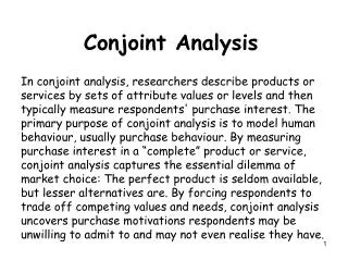
37. CONJOINT ANALYSIS • Conjoint analysis: family of techniques to measure customer preferences, tradeoffs. 37

38. Applications • New product concept identification • Pricing • Benefit segmentation • Competitive analysis • Repositioning or modifying existing products 38

39. Modeling a Single Consumer • Sysco wants to create first class lunch defined on: • Appetizer • a1 = Mushroom tart • a2 = Shrimp cocktail • Salad/Vegetable • b1 = Tossed salad • b2 = Fresh asparagus • Entree • c1 = Fried grouper • c2 = Sole bonne femme 39

40. Goal and Procedure • Goal • Find the combination of appetizer, salad/veggie, and entree that will be most attractive to customers who are buyers at major airlines • Procedure • Customer evaluates subset of combos (15-pt scale) • Estimate “average liking” item effects • Forecast liking of all combos • Design optimal meal for that customer

41. Imagine a customer who obeys an additive model: Overall Liking (ijk) = u a(i) + u b(j) + u c(k) = for Whole Meal Utility / liking for Appetizer (i) + Utility / liking for Salad/Veg (j) + Utility / liking for Entrée (k) And further, suppose: Mushroom tart u (a1) = -2 Shrimp cocktail u (a2) = +2 Salad u (b1) = +1 Asparagus u (b2) = +4 Grouper u (c1) = +4 Sole u (c2) = +6

42. We cannot observe these true utilities (the u’s) directly, but we can observe the overall ratings R(ijk)

43. Notice there is no interaction of preferences across attributes. When this holds, we can get a separate interval scale of “part-utility” from the marginal means for each factor: a + b (part Util) A: R(1..) = 5.5 B: R(.1.) = 6.0 C: R(..1) = 6.5 R(2..) = 9.5 R(.2.) = 9.0 R(..2) = 8.5 1. Because these share a common unit, differences between two levels of factor A can be compared meaningfully to differences between two levels of B and C. Appetizer factor A twice as important as entrée factor C. 2. Because these scales have different and unknown intercepts, we cannot compare the absolute level of one level of factor A to that of a single level of factor B or C. e.g., Though R(2..)= 9.5 for shrimp > R(..2) = 8.5 for sole, u(a2) = +2 for shrimp < u(c2) = +6 for sole. 43

44. Imagine a customer who obeys an additive model: Overall Liking (ijk) = u a(i) + u b(j) + u c(k) = for Whole Meal Utility / liking for Appetizer (i) + Utility / liking for Salad/Veg (j) + Utility / liking for Entrée (k) And further, suppose: Mushroom tart u (a1) = -2 R(1..) = 5.5 Shrimp cocktail u (a2) = +2 R(2..) = 9.5 Salad u (b1) = +1 R(.1.) = 6.0 Asparagus u (b2) = +4 R(.2.) = 9.0 Grouper u (c1) = +4 R(..1) = 6.5 Sole u (c2) = +6 R(..2) = 8.5 44

45. Tradeoffs Which meal would this guy prefer? Option 1 Option 2 Shrimp Cocktail Mushroom Tart Salad Asparagus Grouper Sole

46. Same Conclusions from Subset Critically, we can get the same utility scales if we ask only for a specially chosen subset of all 8 possible combinations: ComboCustomer Rating Mushroom tart, salad, grouper 3 Mushroom tart, asparagus, sole 8 Shrimp cocktail, salad, sole 9 Shrimp cocktail, asparagus, grouper 10 Guess the average evaluation of untested combinations?

47. Goal: Compute expected evaluation of remaining four combos so we can pick the best out of 8. Overall Average? = 7.5 Deviation from 7.5? a1=Mushroom tart Average = 5.5 a2=Shrimp cocktail Average = 9.5 b1=Salad Average = 6.0 b2=Asparagus Average = 9.0 c1=Grouper Average = 6.5 c2=Sole Average = 8.5

48. Now let’s consider how much of a bump up or down we get from the overall average (7.5) for each attribute level. Overall Average? = 7.5 Deviation from 7.5? a1= Mush. Tart Avg = 5.5 5.5 – 7.5 = -2 a2= Shrimp Average = 9.5 9.5 – 7.5 = +2 b1=Salad Average = 6.0 6.0 – 7.5 = -1.5 b2=Asparagus Avg = 9.0 9.0 – 7.5 = +1.5 c1=Grouper Average= 6.5 6.5 – 7.5 = -1 c2=Sole Average = 8.5 8.5 – 7.5 = +1 Compute predicted rating of missing cells by saying: Overall Average + Dev a(i) + Dev b(j) + Dev c(k) e.g., Tart (a1), Salad (b1), Sole (c2) = 7.5 + (-2) + (-1.5) + (+1) = 5

49. What can we conclude? • Best meal? • If you now sell a1, b1, c1, what single change is best? What if you sell a2, b1, c1? • Most important attribute? • Can also cluster individual customers based on their part-utility differences for each attribute to get “benefit segments.” • Can make market share forecasts (next) • Can use for pricing, when price is an attribute