Lavezzo V., Soldati A.

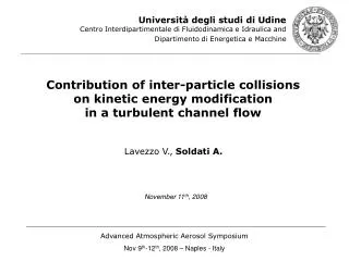
1. Università degli studi di Udine Centro Interdipartimentale di Fluidodinamica e Idraulica and Dipartimento di Energetica eMacchine Contribution of inter-particle collisions on kinetic energy modification in a turbulent channel flow Lavezzo V., Soldati A. November 11th, 2008 Advanced Atmospheric Aerosol Symposium Nov 9th-12th, 2008 – Naples - Italy

2. Influence of inertia and particle-particle collisions… • Tend to decorrelate particles with the coherent eddies that are responsible for their accumulation (Li et al., 2001); • Tend to suppress small wave-lengths in the energy spectrum (Li et al., 2001); • Increase the interaction between particles and carrier fluid (Li et al., 2001); Flow Time Scale, tf Particle Stokes number, St:tp/ tf Particle Relaxation Time, tp = dp2rp/18 m

3. When is it necessary to implement a collision model? Dilute flows vs dense flows (Crowe et al.,1991) Vr 2D D fc= Collision frequency n = particle number density D = particle diameter Vr = particle relative velocity tp = Particle response time tc = Time between collisions DENSE FLOWS dominated by particle collisions DILUTE FLOWS dominated by particle response time

4. Which kind of model can be implemented? • Hard sphere model • Soft sphere model • Type of contact • Particle interactions (coalescence, lubrication force, hydrodynamic interaction, van der Waals forces etc…) Stuttgard University • Single • Multiple • Number of collisions

5. Is it worth to introduce a collision modelin Lagrangian tracking? ADVANTAGES: Simulate a quasi-real problem Consider the effects on particle dispersion and re-suspension in the domain Consider the effects of particles on turbulence DISADVANTAGES: Computational costs increase with the number of particlesNp2 Since a dilute system may not be enough to perceive collision effects in some cases two-way coupling must be taken into account (volume fraction greater than 10-6 Elghobashi et al.,1994)

6. The problem under study…channel flow • Time-dependent 3D turbulent gas flow field with pseudo-spectral DNS • Periodic boundary conditions in the streamwise and spanwise direction (x and y) • No-slip boundary at the wall (z) • Reynolds number: Ret=uth/n=150 • One set of particles p=25 spherical, non-deformable;

7. Particle deposition at the wall • Observations • In channel flow (as well as in pipe flow) particles segregate and accumulate at the wall at different rates depending on their inertia. • Accumulation at the wall is turbulence-induced and is non-uniform. This phenomenon is caused by the preceding vortex that forbids particles to reach the ejection area.

8. Do we need a collision model? Number Concentration St St = 25 St = 5 St = 1 St= 0.2 We can check the overall particle concentration… DILUTE ! …and the local concentration at the wall DENSE !

9. What do we expect if we take collisions into account? Different energy distribution (still to be checked!) The kinetic energy associated with each particle may increase or decrease due to collisions effects. This change will have an impact also on the overall particle energy.

10. What do we expect? Different collision types… Buffer layer Viscous sublayer Wall Viscous sublayer Depending on the relative velocity between the colliding particles: High energy collisions Characterized by possible particle resuspension Low energy collisions Characterized by multiple collision events

11. How to discover if it is true?…Implementing a collision algorithm! • Hard-sphere collision model • Allows for multiple collisions • Pro-active approach in collision detection (Sundaram and Collins, 1996) • i.e.a possible collision is detected at the beginning of the time step and all the particles are advanced using small collision time intervals

12. 1. Searching lattice creation After the new velocity calculation, the domain is divided into several cells according to a fixed criteria: Cell size must be > R + 2% R R = 0.382 wall units (Wang et al.2000) X direction = grid points 1885/128 = 14.71 wall units Y direction = grid points 942/128 = 7.35 wall units Z direction = Grid points = Chebichev polinomials Regular grid spacing = 2h /129

13. 2. Map definition:neighbor list and linked list method The search for possible collisions is restricted to the 26 neighboring cells of the one containing the particle under study. Each cell is numbered from 1 to 128x128x129 and a map is then created. ICELL = 1 + MOD(IX-1+ NX,NX) + MOD(IY-1+ NY,NY)*NX + MOD(IZ-1+ NZ,NZ)*NY*NX Periodic boundaries: IX-1 = NX IX+1 = 1

14. 3.1 Sorting particles in a list Each particle is sorted in a cell according to its position in the domain and a list for each cell is then created. ICELL=1+ MOD(II-1+ NX,NX)+MOD(JJ-1+NY,NY)*NX+MOD(KK-1+NZ,NZ)*NY*NX II : II-1 < Px < II+1 JJ : JJ-1 < Py < JJ+1 KK: KK-1< Pz < KK+1 HEAD(ICELL) = 4 First particle of the chain PARTICLE 1 2 3 4 5 6 7 8 9 10 LIST(I) = 0 1 2 3 0 0 0 0 7 6 Next particle in ICELL No more particles in this cell!

15. 3.2 Sorting particles in a list If a particle is situated in the lowest (kk=1) or in the highest (kk=NZ) cell a mirror particle is then created. A list of the particles in this mirror cell is also created using the method previously described. This is to avoid possible overlaps after wall bouncing!

16. 4. Time to collision calculation Thanks to the lists already created the TIME TO COLLISION for each particle pair is then calculated: The MINIMUM time to collision is then searched and if it is less than the global time step of advancement dt+ the first colliding pair is found! dp Min(t ij ) < dt+

17. 5. Particle advancement to the collision time MIN(tij ) All the particles are advanced to the time to collision tij All the collision time scheduled are updated

18. 6. The velocities of the two colliding particles are then updated and an elastic collision is implemented A solidal reference system with respect to one of the particles is considered and the R rotation matrix is calculated and applied; The new velocities are calculated in the new reference system applying the momentum and energy conservation; The velocities are brought back into the global reference system through the inverse of the R matrix;

19. 7. Post-processing parameters update The approaching angle i.e. the angle between the relative velocity of the two particles and the vector connecting the two centres is calculated; Colliding particle position and velocity is saved; The number of collisions is updated;

20. 9. At the end, after checking for possible overlaps… IF Tcolltot < dt+ Check for possible rebounds at the wall Search for the next scheduled collision and repeat the process IF Tcolltot > dt+ All the particles are advanced in time at the end of the global time step. New rebound control and overlap check is performed.

21. 1. Results: instantaneous particle velocity Low relative velocity High relative velocity

22. 2. Results: collision angle The particle pair that shows higher relative velocity has a colliding angle close to 90 degrees: the particles are approaching almost vertically one another

23. 3. Results: PDF of relative velocity and collision angle Most of the collisions correspond to particle pairs with low relative velocity The collision angle PDF shows almost a gaussian distribution with a mean of 40 degrees

24. 5. Results: particle kinetic energy The particle kinetic energy considering collisions is higher in the channel core. This is due to different particle concentration and simulation times!!!

25. 5. Results: fluid velocity The fluid velocity is unaffected by two-way coupling effects, simulations with collisions are far from being at a stationary point!

26. Conclusions and future developments • A DNS of a turbulent channel flow and Lagrangian particle tracking are considered for particle-particle interaction study; • A collision algorithm with elastic and multiple collisions has been described in detail; • Preliminary results in contrast with the expected division between highly energetic and low energetic collisions, show that most of the particles are colliding with low relative velocity; • Simulations considering particle-particle interactions are still running and need some more time to get appreciable results. How does particle size affect collisions?

27. Acnowledgements: This work has been performed under the Project HPC-EUROPA (RII3-CT-2003-506079), with the support of the European Community - Research Infrastructure Action under the FP6 “Structuring the European Research Area” Programme. The authors would like to thank Prof. Luis Portela and Marcos Cargnelutti (Delft University of Technology) for the useful discussions and helpful technical advices.

28. Seguono slides su PDF accelerazione

29. 5. Results: PDF of particle acceleration streamwise Z+=244 DNS vs experiments As the St number increases the PDF tails become negatively skewed. The shape of the tails in the DNS pdfs differs from the experimental profile

30. What if gravity is turned off? The pdf tails are slightly negatively skewed if gravity is not considered. The St=10.76 particles exhibit a different behavior