Download

1 / 14
150 likes | 415 Vues
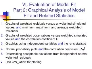
VI. Evaluate Model Fit. Basic questions that modelers must address are: How well does the model fit the data? Do changes to a model, such as reparameterization, actually improve the model fit? What aspects of the model or data need to be changed to improve model fit?

E N D
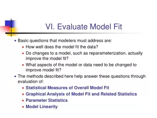
VI. Evaluate Model Fit Basic questions that modelers must address are: How well does the model fit the data? Do changes to a model, such as reparameterization, actually improve the model fit? What aspects of the model or data need to be changed to improve model fit? The methods described here help answer these questions through evaluation of: Statistical Measures of Overall Model Fit Graphical Analysis of Model Fit and Related Statistics Parameter Statistics Model Linearity
VI. Evaluating Model FitPart 1: Statistical Measures of Overall Fit Objective function values Calculated error variance, standard error, and fitted error statistics The AIC and BIC statistics
Objective Function Values • Values of objective functions, such as the weighted least-squares objective function, are a basic measure of model fit. • During regression, the objective is to find the set of parameter values that minimizes the objective function. Ideally, as regression proceeds, the model fit is improved. • Two commonly used objective functions are the weighted least-squares objective function, used in this class, and the maximum likelihood objective function. • Weighted least-squares objective function: where y represents an observed value or a prior value.
Objective Function Values • Maximum likelihood objective function (simplified form): where is the determinant of the weight matrix. • The first term is a function of the total number of observations plus prior values. • The second term is a function of the weighting; for a diagonal weight matrix, the determinant is simply the product of the diagonal elements (the weights). • The third term is the weighted least-squares objective function. • Unlike the weighted least-squares objective function, the maximum likelihood objective function can be negative. • DO EXERCISE 6.1a: Examine objective-function values at the bottom of file ex5.2c.#uout.
Objective Function Values • Values of objective functions, such as the weighted least-squares objective function, are a basic measure of model fit. • During regression, the objective is to find the set of parameter values that minimizes the objective function. Ideally, as regression proceeds, the model fit is improved. • Two commonly used objective functions are the weighted least-squares objective function, used in this class, and the maximum likelihood objective function. • Weighted least-squares objective function: where y represents an observed value or a prior information value. • DO EXERCISE 6.1a: Examine objective-function values.
Calculated Error Variance and Standard Error(Book, p. 95-98) • Problem with using objective function values to assess model fit: They do not account for the negative effects of increasing the number of parameters, and are of limited use in comparing models with different parameterization schemes. • Adding more parameters almost always improves the objective function value, but the parameter estimates become less reliable. • The calculated error variance s2 accounts for the effects of adding more parameters. As NP increases, the denominator decreases, and s2 increases: • The square root of s2 is s, which is the standard error of the regression. • Both s2 and s are dimensionless, and unlike S, can be used to compare the results of models with different parameterizations (but not models with different weighting schemes).
Calculated Error Variance and Standard Error • If the fit achieved by the regression is consistent with the accuracy of the observation data, as expressed by the weighting, then the expected value of both s2 and s is 1.0. • This can be demonstrated using the exercise of Hill and Tiedeman (2007, p. 113-114, exer. 6.1b), which we will not go over in class. • Given that we expect s2 and s to be 1.0 if the model fit is consistent with the observation errors as represented in the weight matrix, deviations from 1.0 can be interpreted in the context of observation error and model error. This insight into model error can be very useful. • The following slides explain how this is done.
Calculated Error Variance and Standard Error • In practice, values for s2 and s often deviate from 1.0. • Significant deviations from 1.0 indicate that the model fit to the observation data is inconsistent with the statistics used to calculate the weights. This doesn’t necessarily mean these statistics are wrong. • Step 1: Test whether s2 significantly deviates from 1.0. Construct a confidence interval for the true error variance: chi-square distribution and define the upper and lower tail values of a chi-square distribution with n degrees of freedom. • Confidence interval on s: take the square root of the limits on s2.
Calculated Error Variance and Standard Error • Interpretation of 95% confidence intervals on s2 : • If the interval includes 1.0, and the weighted residuals are random, then s2 does not significantly deviate from 1.0. The model fit is consistent with the statistics used to calculate the weights. Expressed in terms of probability, there is only a 5% chance that the model fit to the data contradicts the assumptions that (1) the model is reasonably accurate and (2) the statistics used to calculate the weights correctly reflect the observation errors. • If the entire interval is less than 1.0, and the weighted residuals are random, the model fits better than anticipated, based on the weighting used. This is generally not problematic, but is only common in test cases. • If the entire interval is greater than 1.0, then s2 is significantly greater than 1.0, and the model fit is worse than anticipated based on the weighting used. In this situation, the interpretation depends on whether or not the weighted residuals are random.
Calculated Error Variance and Standard Error • If the entire interval > 1.0 and the weighted residuals are random: • Reevaluate the weighting • The weights are calculated using variances, standard deviations, coefficients of variation. • Calculate values of these statistics that are consistent with the model fit. Multiply the variances by s2; the standard deviations and coefficients of variation by s. If the model were re-run with the resulting weights, parameter estimates and residuals would be the same, but s2 would equal 1.0. • If the recalculated statistics can be justified(observation error could be larger than originally assumed), no indication of model error. • If the recalculated statistics cannot be justified, model error may be as much as s times the observation error. There is some indication (Hill+, 1998) that the model error can be correctly represented with common uncertainty measures, but more work is needed to be sure.
Calculated Error Variance and Standard Error • If the entire interval > 1.0 and the weighted residuals are not random: • Significant model error is indicated. Try to find and correct the model error. • Inspect weighted residuals individual and examine spatial and temporal patterns. • Evaluate the model carefully for data input errors and consistency with independent information about the system.
Fitted Error Statistics (Book, p. 95-96) • s and s2 are dimensionless. Difficult to convey goodness of fit to others using dimensionless numbers. • Fitted error statistic (not standard statistical terminology) reflects model fit in the same units as one type of observation. • Calculation: s × (std dev) or (coef of var) used to define weights for a group of observations. • Fitted standard deviation, on average, the difference between simulated values and observations for the group. • For a few observations, just report the weighted residuals • DO EXERCISE 6.1c: Evaluate calculated error variance, standard error, and fitted error statistics. For fitted error to heads, compare to overall head loss in the system.
AIC and BIC Statistics • AIC (Akaike’s Index Criteria), AICc, and BICmore strongly account for the negative effect of increasing the number of estimated parameters when comparing alternative models. • Smaller values indicate better models. • Start with the maximum-likelihood objective function, S’ and add one or two terms that are a function of the number of parameters: Use AICc if NOBS/NP<40 • DO EXERCISE 6.1d: Examine the AIC and BIC statistics.
New exercise These figures show the value of the added terms given different numbers of observations and parameters. Based on theory:BIC uses additional data to focus in on an existing model with fewer parameters, while AIC and AICc is more likely to choose a model with more parameters when there are more data. How do these graphs support or refute the theory?