Active Lighting for Appearance Decomposition
Active Lighting for Appearance Decomposition. Todd Zickler DEAS, Harvard University. I = f ( shape,. reflectance ). illumination,. ?. f -1 ( I ) =. Appearance. Research Overview. COLOR IMAGE FILTERING. 3D RECONSTRUCTION. APPEARANCE CAPTURE. PHOTOMETRIC INVARIANTS. ?.

Active Lighting for Appearance Decomposition
E N D
Presentation Transcript
Active Lighting for Appearance Decomposition Todd Zickler DEAS, Harvard University
I = f (shape, reflectance) illumination, ? f -1( I ) = Appearance Appearance Decomposition
Research Overview COLOR IMAGE FILTERING 3D RECONSTRUCTION APPEARANCE CAPTURE PHOTOMETRIC INVARIANTS Appearance Decomposition
? f -1( I ) = I = f (shape, reflectance, illumination) Getting 3D Shape:Image-based Reconstruction Appearance Decomposition
Reflectance: BRDF Bi-directional Reflectance Distribution Function Appearance Decomposition
LAMBERTIAN: IDEALLY DIFFUSE Conventional 3D Reconstruction:Restrictive Assumptions Appearance Decomposition
Example: Conventional Stereo Il Ir ASSUMPTION: Il = Ir Appearance Decomposition
Example: Conventional Stereo Il Ir ASSUMPTION: Il = Ir Appearance Decomposition
Conventional 3D Reconstruction:Restrictive Assumptions Variational Stereo [Faugeras and Keriven, 1998] Shape from shading [Tsai and Shaw, 1994] Multiple-window stereo [Fusiello et al., 1997] Space Carving [Kutulakos and Seitz, 1998] Appearance Decomposition
Reflectance: BRDF Appearance Decomposition
Reflectance: BRDF Appearance Decomposition
Helmholtz Reciprocity [Helmholtz 1925; Minnaert 1941; Nicodemus et al. 1977] Appearance Decomposition
Stereo vs. Helmholtz Stereo STEREO HELMHOLTZ STEREO Appearance Decomposition
Stereo vs. Helmholtz Stereo STEREO HELMHOLTZ STEREO Appearance Decomposition
Stereo vs. Helmholtz Stereo STEREO HELMHOLTZ STEREO Appearance Decomposition
Il Ir • Specularities “fixed” to surface • Relation between Il and Ir independent of BRDF Reciprocal Images Appearance Decomposition
p ^ ^ vr vr ^ ^ n n ol or ^ ^ vl vl = Reciprocity Constraint p ol or Appearance Decomposition
p p ^ ^ vr vr ^ ^ n n ol or ol or • Arbitrary reflectance • Surface normal ^ ^ vl vl = Reciprocity Constraint Appearance Decomposition
Reciprocal Acquisition CAMERA LIGHT SOURCE Appearance Decomposition
Recovered Normals [Zickler et al. 2002] Appearance Decomposition
Recovered Surface [Zickler et al., ECCV 2002] Appearance Decomposition
In Practice • Arbitrary Reflectance • Off-the-shelf components • Direct surface normals • Images aligned with recovered shape • Self-calibrating (coming…) Appearance Decomposition
Ongoing Work: Auto-calibration [Zickler et al., CVPR 2003, CVPR 2006,…] Appearance Decomposition
Research Overview COLOR IMAGE FILTERING 3D RECONSTRUCTION APPEARANCE CAPTURE PHOTOMETRIC INVARIANTS Appearance Decomposition
DIFFUSE SPECULAR = + Reflectance Decomposition [Phong 1975; Shafer, 1985] Appearance Decomposition
Reflectance Decomposition [Shafer, 1985] Appearance Decomposition
= + LAMBERTIAN: IDEALLY DIFFUSE Reflectance Decomposition: Simplifies the Vision Problem = + Appearance Decomposition
Reflectance Decomposition: A Difficult Inverse Problem DIFFUSE SPECULAR = + = + [Bajscy et al., 1996; Criminisi et al., 2005; Lee and Bajscy, 1992; Lin et al., 2002; Lin and Shum, 2001; Miyazaki et al., 2003; Nayar et al., 1997; Ragheb and Hancock, 2001; Sato and Ikeutchi, 1994; Tan and Ikeutchi, 2005; Wolfe and Boult, 1991,…] Appearance Decomposition
Known Illuminant: Still Ill-posed B S IRGB D? G R Appearance Decomposition
Known Illuminant: Still Ill-posed B S IRGB D? G R Appearance Decomposition
Observation:Explicit Decomposition not Required B S IRGB r1 G r2 J • INVARIANT TOSPECULAR REFLECTIONS • BEHAVES ‘LAMBERTIAN’ R Appearance Decomposition
B S IRGB r1 G r2 J R Observation:Explicit Decomposition not Required IRGB || J || [Mallick, Zickler, Kriegman, Belhumeur, CVPR 2005] Appearance Decomposition
Generalization: Mixed Illumination SINGLE ILLUMINANT MIXED ILLUMINATION B B S1 S S2 IRGB IRGB r1 G G r2 J r1 J R R [Zickler, Mallick, Kriegman, Belhumeur, CVPR 2006] Appearance Decomposition
Generalization: Mixed Illumination Appearance Decomposition
Example: Binocular Stereo Conventional Grayscale(R+G+B)/3 Specular Invariant, ||J||(blue illuminant) Specular Invariant, ||J||(blue & yellow illuminants) One image from input stereo pair Recovered depth [Algorithm: Boykov, Veksler and Zabih, CVPR 1998] Appearance Decomposition
Example: Optical Flow Conventional Grayscale(R-+G+B)/3 Specular Invariant, ||J||(blue illuminant) Specular Invariant, ||J||(blue & yellow illuminants) Ground truth flow [Algorithm: Black and Anandan, 1993] Appearance Decomposition
Example: Photometric Stereo J behaves ‘Lambertian’ Linear function of surface normal [Mallick, Zickler, Kriegman, Belhumeur, CVPR 2005] Appearance Decomposition
Example: Photometric Stereo J behaves ‘Lambertian’ Linear function of surface normal [Mallick, Zickler, Kriegman, Belhumeur, CVPR 2005] Appearance Decomposition
Example: Photometric Stereo J behaves ‘Lambertian’ Linear function of surface normal [Mallick, Zickler, Kriegman, Belhumeur, CVPR 2005] Appearance Decomposition
Example: Photometric Stereo [Mallick, Zickler, Kriegman, Belhumeur, CVPR 2005] Appearance Decomposition
Example: Photometric Stereo [Mallick, Zickler, Kriegman, Belhumeur, CVPR 2005] Appearance Decomposition
ψ Generalized Hue B S IRGB r1 G r2 J R Appearance Decomposition
Example: Material-based Segmentation Conventional Grayscale Specular Invariant ||J|| Input image Generalized Hue y Conventional Hue [Zickler, Mallick, Kriegman, Belhumeur, CVPR 2006] Appearance Decomposition
Active Lighting for Image-guided Surgery? Endoscopic imagery: • Illuminant(s) is/are controlled and known • Non-Lambertian surfaces • Lack of texture Active lighting can provide: • Precise shape (surface normals) for a broad class of (non-Lambertian) surfaces • Specular and/or shading invariance (e.g., optical flow, tracking, segmentation) • Minimal hardware requirements Appearance Decomposition
Acknowledgements Satya Mallick, UCSD Peter Belhumeur, Columbia University David Kriegman, UCSD Sebastian Enrique, Columbia University Ravi Ramamoorthi, Columbia University zickler@eecs.harvard.edu http://www.eecs.harvard.edu/~zickler Appearance Decomposition