Active Appearance Models

1. Active Appearance Models based on the article: T.F.Cootes, G.J. Edwards and C.J.Taylor. "Active Appearance Models", 1998. presented by Denis Simakov

2. Mission • Image interpretation by synthesis • Model that yields photo-realistic objects • Rapid, accurate and robust algorithm for interpretation • Optimization using standard methods is too slow for realistic 50-100 parameter models • Variety of applications • Face, human body, medical images, test animals

3. Building an Appearance Model

4. Appearance • Appearance = Shape + Texture • Shape: tuple of characteristic locations in the image, up to allowed transformation • Example: contours of the face up to 2D similarity transformation (translation, rotation, scaling) • Texture: intensity (or color) patch of an image in the shape-normalized frame, up to scale and offset of values

5. Shape • Configuration of landmarks • Good landmarks – points, consistentlylocated in every image. Add also intermediate points • Represent by vector of the coordinates:e.g. x=(x1,...,xn, y1,...,yn)T for n 2D landmarks • Configurations x and x' are considered to have the same shape* if they can be merged by an appropriate transformation T (registration) • Shape distance – the distance after registration: * Theoretical approach to shape analysis: Ian Dryden (University of Nottingham)

6. warped to becomes Shape-free texture • An attempt to eliminate texture variation due to different shape (“orthogonalization”) • Given shape x and a target “normal” shape x' (typically the average one) we warp our image so that points of x move into the corresponding points of x'

7. Modeling Appearance training set (annotated grayscale images) shape (tuple of locations) texture (shape-free) PCA PCA model of shape model of texture PCA model of appearance

8. * Training set • Annotated images • Done manually, it is the most human time consuming anderror prone part of building the models • (Semi-) automatic methods are being developed** * Example from: Active Shape Model Toolkit (for MATLAB), Visual Automation Ltd. ** A number of references is given in: T.F.Cootes and C.J.Taylor. “Statistical Models of Appearance for Computer Vision”, Feb 28 2001; pp. 62-65

9. Training sets for shape and texture models • From the initial training set (annotated images) we obtain {x1,...,xn} – set of shapes, {g1,...,gn} – set of shape-free textures. • We allow the following transformations: • S for the shape: translation (tx,ty), rotation , scaling s. • T for the texture: scaling , offset  (Tg = (g – 1)/). • Align both sets using these transformations, by minimizing distance between shapes (textures) and their mean • Iterative procedure: align all xi (gi) to the current ( ), recalculate ( ) with new xi (gi), repeat until convergence.

10. Examples of training sets Shapes Textures * The mean shape * From the work of Mikkel B. Stegmann, Section for Image Analysis, The Technical University of Denmark

11. Example: 3 modes of a shape model Model of Shape • Training set {x1,...,xn} of aligned shapes • Apply PCA to the training set • Model of shape: where (the mean shape) and Ps (matrix of eigenvectors) define the model; bs is a vector of parameters of the model. • Range of variation of parameters: determined by the eigenvalues, e.g.

12. Example: 1st mode of a texture model: Model of Texture • Training set {g1,...,gn} of shape-free normalized image patches • Apply PCA • Model of texture: • Range of variation of parameters

13. Combining two models • Joint parameter vectorwhere the diagonal matrix Wsaccounts for different units of shape and texture parameters. • Training set • For every pair (xi,gi) we obtain: • Apply PCA to the training set {b1,...,bn} • Model for parameters: b = Pcc, Pc = [Pcs|Pcg]T • Finally, the combined model: where Qs = PsWs-1Pcs, Qs = PgPcg.

14. Tim Cootes His shape A mode of the model • Color model (by Gareth Edwards) Several modes Examples (combined model) • Self-portrait of the inventor

15. Exploiting an Appearance Model

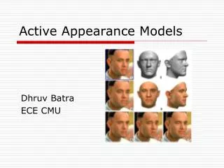
16. Generating synthetic images: example By varying parameters c in the appearance model we obtain synthetic images:

17. Given: • an appearance model, • a new image, • a starting approximation Find: the best matching synthetic image Active Appearance Model (AAM) • Difference vector: dI = Ii – Im • Ii – input (new) image; • Im – model-generated (synthetic) image for the current estimation of parameters. • Search for the best match • Minimize D = |dI|2, varying parameters of the model Approach:

18. Predicting difference of parameters • Knowing the matching error dI, we want to obtain information how to improve parameters c • Approximate this relation by dc = AdI • Precompute A: • Include into dc extra parameters: translations, rotations and scaling of shape; scaling and offset of gray levels (texture) • Take dI in the shape-normalized framei.e. dI = dg where textures are warped into the same shape • Generate pairs (dc,dg) and estimate A by linear regression.

19. Translation along one axis In the multi-resolution model (L0 – full resolution, L1 and L2 – succesive levels of the Gaussian pyramid) Checking the quality of linear prediction We can check our linear prediction dc = Adg by perturbing the model

20. AAM Search Algorithm Iterate the following: For the current estimate of parameters c0 • Evaluate the error vector dg0 • Predict displacement of the parameters: dc = Adg0 • Try new value c1 = c0 – kdc for k=1 • Compute a new error vector dg1 • If |dg1|<|dg0| then accept c1 as a new estimate • If c1 was not accepted, try k=1.5; 0.5; 0.25, etc. until |dg| is no more improved. Then we declare convergence.

21. Model of face Model of hand From the work of Mikkel B. Stegmann, Section for Image Analysis, The Technical University of Denmark AAM search: examples

22. Extension of AAM By Jörgen Ahlberg, Linköping University AAM: tracking experiments AAM Done with AAM-API (Mikkel B. Stegmann)

23. AAM: measuring performance • Model, trained on 88 hand labeled images (about 200 pixels wide), was tested on other 100 images. Convergence rate Proportion of correct convergences

24. View-Based Active Appearance Models based on the article: T.F. Cootes, K.N. Walker and C.J.Taylor, "View-Based Active Appearance Models", 2000. presented by Denis Simakov

25. View-Based Active Appearance Models Basic idea: to account for global variation using several more local models. For example: to model 180 horizontal head rotation exploiting models, responsible for small angle ranges

26. ±(40- 60) -40- +40 ±(60- 110) View-Based Active Appearance Models • One AAM (Active Appearance Model) succeeds to describe variations, as long as there no occlusions • It appears that to deal with 180 head rotation only 5 models suffice (2 for profile views, 2 for half-profiles, 1 for the front view) • Assuming symmetry, we need to build only 3 distinct models

27. Estimation of head orientation where  is the viewing angle, c – parameters of the AAM; c0, cc and cs are determined from the training set • Assumed relation: • For the shape parameters this relation is theoretically justified; for the appearance parameters its adequacy follows from experiments • Determining pose of a model instance • Given c we calculate the view angle : where is the pseudo-inverse of the matrix [cc|cs]T

28. Tracking through wide angles Given several models of appearance, covering together a wide angle range, we can track faces through these angles • Match the first frame to one of the models (choose the best). • Taking the model instance from the previous frame as the first approximation, run AAM search algorithm to refine this estimation. • Estimate head orientation (the angle). Decide if it’s time to switch to another model. • In case of a model change, estimate new parameters from the old one, and refine by the AAM search. To track a face in a video sequence:

29. Tracking through wide angles: an experiment • 15 previously unseen sequences of known people (20-30 frames each). • Algorithm could manage 3 frames per second (PIII 450MHz)

30. Predicting new views • Given a single view of a face, we want to rotate it to any other position. • Within the scope of one model, a simple approach succeeds: • Find the best match c of the view to the model. Determine orientation . • Calculate “angle-free” component: cres = c – (c0+cccos()+cssin()) • To reconstruct view at a new angle , use parameter:c() = c0+cccos()+cssin() + cres

31. Predicting new views: wide angles • To move from one model to another, we have to learn the relationship between their parameters • Let ci,j be the “angle-free” component (cres) of the i’th person in the j’th model (an average one). Applying PCA for every model, we obtain: ci,j = cj+Pjbi,jwhere cj is the mean of ci,j over all people i. • Estimate relationship between bi,j for different models j and k by linear regression:bi,j = rj,k+Rj,kbi,k • Now we can reconstruct a new view: ...

32. Predicting new views: wide angles (cont.) • Now, given a view in model 1, we reconstruct view in model 2 as follows: • Remove orientation: ci,1 = c – (c0+cccos()+cssin()) • Project into the space of principle components of the model 1: bi,1 = P1T(ci,1 – c1). • Move to the model 2: bi,2 = r2,1+R2,1bi,1. • Find the “angle-free” component in the model 2:ci,2 = c2+P2bi,2. • Add orientation: c() = c0+cccos()+cssin() + ci,2.

33. Predicting new views: example • Training set includes images of 14 people. • A profile view of unseen person was used to predict half-profile and front views.