FINC4101 Investment Analysis

1. FINC4101 Investment Analysis Instructor: Dr. Leng Ling Topic: Portfolio Theory I

2. Learning objectives • Compute different measures of investment performance: • Holding-period return (HPR) • Arithmetic average • Geometric average • Dollar-weighted return • Compute the expected return, variance and standard deviation of a risky investment.

3. Concept Map

4. Portfolio Theory I: Concept Map

5. Investment return over 1 period: Holding period return (HPR) • Rate of return over a given investment (holding) period.Has two components: • Price change = ending price – beginning price • Cash income

6. Holding period return (HPR) • Assumes that cash income is paid at the end of the holding period. • If cash income is received earlier, reinvestment income is ignored. • HPR can be used for different types of investments: stock, bond, mutual fund etc. • For stock, cash income = dividend • For bond, cash income = coupon

7. Holding period return (HPR) • Stock

8. Simple HPR example • You are thinking of investing in ABC Inc’s stock. You intend to hold the stock for 1 year. ABC’s stock is currently selling at $50 and is expected to rise to $56 by the end of the year. The company is expected to pay a per share dividend of $0.60 during the year. Compute: • HPR • Capital gains yield • Dividend yield. • Sum up the capital gains yield and the dividend yield. Is that the same as the HPR?

9. Investment return over many periods • Three alternative ways of measuring average returns over multiple periods: • Arithmetic average (arithmetic mean) • Geometric average (geometric mean) • Dollar-weighted return • Use the following example to illustrate each return measure.

10. Example: Table 5.1 • Quarterly cash flows and HPRs of a mutual fund. What is the arithmetic average, geometric average and dollar-weighted return over the four quarters?

11. Arithmetic average • Suppose we hold an asset over N periods: 1, 2,…, and N. • And we label the HPR in each period as: r1, r2, …, rN • The arithmetic average is the sum of returns in each period divided by number of periods. Arithmetic average= (r1 + r2 + r3 + ... rN) /N • In the example,arithmetic average = (10+25-20+25)/4 = 10%

12. Geometric Average (time-weighted) • Single per period return that gives the same cumulative performance as the sequence of actual returns. Geometric average = [(1+r1) x (1+r2) ... x (1+rN)]1/N - 1 • In the example, geometric average= [(1.1) x (1.25) x (.8) x (1.25)] 1/4 - 1 = (1.375) 1/4 -1 = .0829 = 8.29%

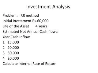
13. Dollar-weighted return (IRR) • This is simply the internal rate of return (IRR) on an investment ! • IRR: the interest rate that will make the PV of cash inflows equal to the PV of cash outflows. • In other words, IRR is the discount rate such that the NPV is 0.

14. Dollar-weighted return (IRR) • In the example, think in terms of capital budgeting. So, the mutual fund is a “project” from investor’s perspective. • Initial Investment is an outflow • Ending value is an inflow • Additional investment is an outflow • Reduced investment (withdraw money) is an inflow

15. Dollar-Weighted Return Using the definition of the IRR,

16. Quoting Rates of Return Annual percentage rate, APR = rate per period X n Where n = no. of compounding periods per year Effective annual interest rate, EAR

17. Quoting Rates of Return • With continuous compounding, the relationship between EAR and APR becomes EAR = eAPR – 1 ‘e’ is the exponential function (that appears on your financial calculator as [ex]) Equivalently, APR = Ln(1 + EAR) Ln is the natural log function.

18. HPR, APR, EAR problem • Suppose you buy a bond of General Electric at a price of $990. The bond pays coupons semi-annually, has an annual coupon rate of 6%, a face value of $1,000 and will mature in six months’ time. You intend to hold the bond till it matures. • What is the 6-month HPR? • What is the APR of this investment? • What is the EAR of this investment?

19. Another example of HPR • Suppose you bought a bond of General Electric at a price of $990 6 months ago. The bond pays coupons semi-annually, has an annual coupon rate of 6%, a face value of $1,000 and will mature in 12 months from today. Today it just paid the coupon and you intend to sell it immediately at current market price. The current YTM is 15%. • What is the current market price? • What will be your HPR?

20. Describing investment uncertainty: Scenario analysis • Investment is risky simply because we don’t know what will happen in the future for certain. One way of quantifying risk is through scenario analysis. • Scenario analysis: The process of devising a list of possible economic scenarios and specifying: - • The likelihood (probability) of each scenario. • The HPR that will be realized in each scenario. • The list of possible HPRs with associated probabilities is called the probability distribution of HPRs. This is critical in helping us to evaluate risky investments.

21. Probability distribution of HPR • The probability distribution provides information for us to measure the reward and risk of an investment. • Reward of the investment: Expected return • Also known as ‘mean return’, ‘mean of the distribution of HPRs’. • Risk of the investment: Variance Let’s start with a simple scenario analysis.

22. Say you want to buy Google’s stock and hold it for a year. • During this coming year, you think there are 3 possible economic scenarios: boom, normal growth, recession.

23. Expected Return, E(r) • The weighted average of returns in all possible scenarios, s = 1,2,…S, with weightsequal to the probability of that particular scenario. p(s): probability of scenario s r(s): HPR in scenario s

24. Expected Return, E(r) • With the formula, Google’s expected return is: E(r) = (0.25 x 44) + (0.5 x 14) + (0.25 x -16) = 14% Probability in each scenario HPR in each scenario

25. Variance, Var(r) • When we talk about risk, we often think of surprises or deviations from what we expect. Variance captures this idea. • Variance: The expected value of squared deviation from the mean. • Also known as σ2 (read as ‘sigma squared’).

26. Standard deviation, SD(r) Standard deviation: Square root of variance Returning to the Google example, Var(r) = 0.25(44 – 14)2 + 0.5(14 – 14)2 + 0.25(-16 -14)2 = 450 SD(r)= (450)1/2 = 21.21%

27. How to interpret E(r), Var(r) and SD(r) • The bigger the expected return, the bigger the potential reward from the investment, vice versa. • The bigger the variance, the bigger the risk of the investment, vice versa. • The bigger the standard deviation, the bigger the risk of the investment, vice versa.

28. Describing investment performance in the past • If we are interested in the rewards from investing in the past (using historical data), we can use (1) arithmetic average, (2) geometric average. • To quantify risk, use ‘historical’ or ‘sample’ variance: Arithmetic average No. of periods

29. Example: S&P500 index, 1988-1992 Compute the arithmetic average, geometric average, and variance.

30. Example: S&P500 index, 1988-1992

31. Example: S&P500 index, 1988-1992, cont’d Arithmetic average = 83.4/5 =16.7% Geometric average = [(1.169) x (1.313) x (0.968) x (1.307) x (1.077)]1/5 – 1 = 0.15902 or 15.9% Variance = 886.21/(5 – 1) = 221.6 Standard deviation = (221.6)1/2 =14.9%

32. Risk premiums & risk aversion • If you don’t want to invest in a risky asset like a stock, what is the alternative? • Risk-free assets like treasury bills. The return you get is the risk-free rate (rf). • Risk-free rate = rate of return that can be earned with certainty. • Risk premium: expected return in excess of the risk-free rate. Risk premium = E(r) – rf

33. Risk premium depends on risk aversion and variance • Risk aversion: reluctance to accept risk. • Risk premium of a portfolio, E(rp) – rf is E(rp) – rf= ½ x A x var(rp) A = measures degree of risk aversion, Var(rp) = variance (risk) of the portfolio Risk premium increases if: • Portfolio variance increases OR • Risk-aversion, A, increases

34. the average A in market = ?

35. Sharpe Ratio • Measure the risk-return tradeoff is the standard deviation of excess returns. * It works for portfolio only, not individual security.

36. Problem sets after Chapter 5, # 11. • The expected cash flow is: (0.5 x $50,000) + (0.5 x $150,000) = $100,000 With a risk premium of 10%, the required rate of return is 15%. Therefore, if the value of the portfolio is X, then, in order to earn a 15% expected return: X(1.15) = $100,000  X = $86,957 • If the portfolio is purchased at $86,957, and the expected payoff is $100,000, then the expected rate of return, E(r), is: = 0.15 = 15.0% The portfolio price is set to equate the expected return with the required rate of return. • If the risk premium over T-bills is now 15%, then the required return is: 5% + 15% = 20% The value of the portfolio (X) must satisfy: X(1.20) = $100, 000  X = $83,333 • For a given expected cash flow, portfolios that command greater risk premium must sell at lower prices. The extra discount from expected value is a penalty for risk.

37. Summary • Single period: holding-period return (HPR) • Many periods: arithmetic average, geometric average, and dollar-weighted return. • Expected return measures the ‘reward’ from an investment. • Variance (standard deviation) measures the ‘risk’ from an investment.

38. Practice 1 1.Chapter 5 problem sets (p.139): 5,6,7,8. 2. Suppose you bought a bond of BT Co. at a price of $990 6 months ago. The bond pays coupons semi-annually, has an annual coupon rate of 6%, a face value of $1,000 and will mature in 24 months from today. Today it just paid the coupon. The current YTM is 15%. • What is the current market price? What is your HPR for the last 6 months? • If the interest rate on the market (YTM) does not change for the next 2 years, what will be your HPR for one year if you intend to sell the bond after 6 months receiving the 2nd coupon payment? (assume all coupons do not earn any investment returns)

39. Homework 1 1. Suppose an investor’s risk aversion A=2 and the variance of the return of the portfolio he chose is 0.0260. The risk-free rate is 2%. The value of the portfolio has 0.3 probability to go to $2000 in one year, 0.5 probability to $1500 and 0.2 probability to $1000. What is the maximum price he would pay for this portfolio? 2. Suppose you bought a bond at a price of $990 12 months ago. The bond pays coupons annually, has an annual coupon rate of 6%, a face value of $1,000 and will mature in 36 months. Today it just paid the coupon. The current YTM is 15%. Suppose the YTM will decrease to 10% after 12 months and then remains the same till expiration. What is the arithmetic average annual return for the next two years?