Download
1 / 27
270 likes | 405 Vues
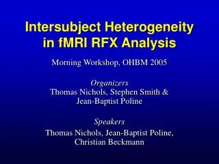
Intersubject Heterogeneity in fMRI RFX Analysis. Morning Workshop, OHBM 2005 Organizers Thomas Nichols, Stephen Smith & Jean-Baptist Poline Speakers Thomas Nichols, Jean-Baptist Poline, Christian Beckmann. Distribution of each subject’s estimated effect. Fixed vs. Random Effects in fMRI.

E N D
Intersubject Heterogeneity in fMRI RFX Analysis Morning Workshop, OHBM 2005 OrganizersThomas Nichols, Stephen Smith &Jean-Baptist Poline Speakers Thomas Nichols, Jean-Baptist Poline, Christian Beckmann
Distribution of each subject’s estimated effect Fixed vs.RandomEffects in fMRI 2FFX Subj. 1 Subj. 2 • Fixed Effects • Intra-subject variation suggests all these subjects different from zero • Random Effects • Intersubject variation suggests population not very different from zero Subj. 3 Subj. 4 Subj. 5 Subj. 6 0 2RFX Distribution of population effect
Multisubject fMRI Analyses • Fixed Effects Analyses • Compare effect magnitude to scan-to-scan variation, measurement error • Inferences only suitable for that cohort • Random Effects (RFX) analyses • Compare effect magnitude to combination of scan-to-scan & subject-to-subject • Inferences can be generalized to the population sampled(Assuming you have a random sample from the population of interest!)
RFX Analyses Assumptions • 2nd level parametric models make more assumptions! • 1st level: Measurement error Normal • 2nd level: True subject responses Normal • Normality needed for... • Optimally precise estimates • Accurate P-values & thresholds
Normality means... • Symmetric • No skew • Unimodal • No mixtureof populations • Thin tails • No outliers
But Non-Normality may be interesting! • Bimodality • In controls, two populations of responses could be explained by behavior differences • In patients, could point to disease sub-groups • Outliers • Exceptional individuals could be performing task in completely different manner • All different aspects of heterogeneity ...
Purpose of Workshop • Raise awareness of heterogeneity in group analyses • Talk 1: Traditional assumption checking Thomas Nichols, University of Michigan • Talk 2: Finding unusual subjects, multivariately Jean-Baptist Poline, CEA- SHFJ • Talk 3: Finding multivariate structure without models Christian Beckmann, Oxford University
Massively UnivariateModel Diagnosis forGroup fMRI Data Thomas Nichols Department of Biostatistics, University of Michigan joint withHui Zhang, University of Michigan Wen-Lin Luo, Merck & Co, Inc http://www.sph.umich.edu/~nichols OHBM Morning Workshop June 14, 2005
Statistical Commandments • But its not easy with imaging data! • 100,000 voxels, 1,000 scans, 20 subjects • Look at all 2 billion data points!? • Check all 100,000 models? • Thou shalt look at your data • Thou shalt check your assumptions
Our Solution • Decompose data into signal & noise Y = X + and explore each, using... • Model and scan summaries • Each sensitive to different violations of assumptions • Dynamic graphical tool • Explore many summaries simultaneously • Efficiently jump from summary to raw or residual data • End Result • Swiftly localize and understand problems
Linear model fit at each voxel Assumptions on errors Data = TrueFit + RandomError = EstimatedFit + Residuals X y = X + = + e Plot e vs X, X, anything Methods: Model Checked with residuals e Mean 0, Constant Var.E(i)=0, Var(i)=2 UncorrelatedCov(i,j)=0 Plot ei vs ei+1, spectrum NormalityP(i x) = (x) QQ plot, e(i) vs. E(z(i))
Methods: Model Summaries • Create images of diagnostic statistics
Methods:Scan Summaries • No spatial model explicitly fit • But several ad hoc measures useful
Scan Summaries • Parallel time series w/ cursor Scan Summaries Scan Summaries Model Summaries Model Summaries • Model Summaries • Orthogonal Slice Viewers, MIPs • Model Detail • Raw data, fitted & residualtime series, and diagnostic plots Scan Detail • Scan Detail • Series of standardized residualimages Model Detail Model Detail Scan Detail Methods: Graphical Tool
Methods: General Strategies • Scan Summaries • One bad subject? Several? • Model Summaries • Explore noise & signal • Assess assumptions w/ diagnostics • Find problem voxels • Model Detail • For a problem voxel, find which subjects involved • Model Detail • For a problem subject, assess spatial extent of problem
Data: FIAC Data • Acquisition • 3 TE Bruker Magnet • For each subject:2 (block design) sessions, 195 EPI images each • TR=2.5s, TE=35ms, 646430 volumes, 334mm vx. • Experiment (Block Design only) • Passive sentence listening • 22 Factorial Design • Sentence Effect: Same sentence repeated vs different • Speaker Effect: Same speaker vs. different • Analysis • Slice time correction, motion correction, sptl. norm. • 555 mm FWHM Gaussian smoothing • Box-car convolved w/ canonical HRF • Drift fit with DCT, 1/128Hz
Look at the Data! • With small n, really can do it! • Start with anatomical • Alignment OK? • Yup • Any horrible anatomical anomalies? • Nope
Look at the Data! • Mean & Standard Deviationalso useful • Variancelowest inwhite matter • Highest around ventricles
Look at the Data! • Then the functionals • Set same intensity window for all [-10 10] • Last 6 subjects good • Some variability in occipital cortex
Feel the Void! • Compare functional with anatomical to assess extent of signal voids
Check Scan Summaries • Not so interesting but... • Note subject 9 (FIAC8) has 1% outliers
Check Model Summaries Tstat Con. • Expected signal • Auditory cortex in both T& con • Unexpected structure • Stdev shows visual cortex,MCA variability Stdev Norm.Test Out-liers
Check Model Detail • Visual cortex variable, especially in subj 2, 8, 9, 10
Check Model Detail • Normality test big in cingulate • Subject 9 again!
Check Scan Detail • Standardized residuals confirm subject 9 is weird • Ant/Superior Cingulate deactivated(in addition to V1)
Conclusions • Group data should be explored • To understand anomalies • To generate new hypotheses • Assumptions must be checked • For unbiased and optimal estimates • For valid p-values • Assumptions in group fMRI can be checked efficiently • Model and scan diagnostic summaries • Explore with dynamic visualization software • Localize and understand artifacts • Software: Statistical Parametric Mapping Diagnosis • http://www.sph.umich.edu/~nichols/SPMd • Luo & Nichols, NeuroImage, 2003, 19(3):1014-1032