FMRI Connectivity Analysis in AFNI
350 likes | 375 Vues
Learn about FMRI connectivity analysis techniques, including correlation analysis, SEM, model validation, Granger causality, and more. Understand how to interpret and avoid pitfalls in correlation vs. causation in brain connectivity studies.

FMRI Connectivity Analysis in AFNI
E N D
Presentation Transcript
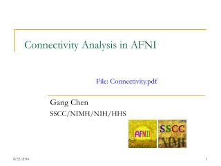
FMRI Connectivity Analysis in AFNI Gang Chen SSCC/NIMH/NIH
Structure of this lecture • Overview • Correlation analysis • Simple correlation • Context-dependent correlation (PPI) • Structural equation modeling (SEM) • Model validation • Model search • Granger causality (GC) • Bivariate: exploratory - ROI search • Multivariate: validating – path strength among pre-selected ROIs
Overview: FMRI connectivity analysis • All about FMRI • Not for DTI • Some methodologies may work for MEG, EEG-ERP • Information we have • Anatomical structures • Seed-based: A seed region in a network, or • Network-based: A network with all relevant regions known • Brain output (BOLD signal): regional time series • What can we say about inter-regional communications? • Inverse problem: make inference about intra-cerebral neural processes from extra-cerebral/vascular signal • Based on response similarity (and sequence)
Approach I: seed-based; ROI search • Regions involved in a network are unknown • Bi-regional (seed vs. whole brain) (3d*): brain volume as input • Mainly for ROI search • Popular name: functional connectivity • Basic, coarse, exploratory with weak assumptions • Methodologies: simple correlation, PPI, bivariate GC • Weak interpretation: may or may not indicate directionality/causality
Approach II: network-based • Regions in a network are known • Multi-regional (1d*): ROI data as input • Model validation, connectivity strength testing • Popular name: effective or structural connectivity • Strong assumptions: specific, but with high risk • Methodologies: SEM, multivariate GC, DCM • Directionality, causality (?)
Interpretation Trap: Correlation vs. Causation! • Some analyses require fine time resolution we usually lack • Path from (or correlation btw) A to (and) B doesn’t necessarily mean causation • Bi-regional approach simply ignores the possibility of other regions involved • Analysis invalid if a relevant region is missing in a multi-regional model • Robust: connectivity analysis < regression analysis • Determinism in academics and in life • Linguistic determinism: Sapir-Whorf hypothesis (Adopted from http://xkcd.com/552/)
Preparatory Steps • Warp brain to standard space • adwarp, @auto-tlrc, align_epi_anat.py • Create ROI • Sphere around a peak activation voxel: 3dUndump –master … –srad … • Activation cluster-based (biased unless from independent data?): localizer • Anatomical database • Manual drawing • Extract ROI time series • Average over ROI: 3dmaskave –mask, or 3dROIstats –mask • Principal component among voxels within ROI: 3dmaskdump, then 1dsvd • Seed voxel with peak activation: 3dmaskdump -noijk -dbox • Remove effects of no interest • 3dSynthesize and 3dcalc • 3dDetrend –polort • RETROICORR/RetroTS.m • 3dBandpass
Simple Correlation Analysis • Seed vs. rest of brain • ROI search based on response similarity • Looking for regions with similar signal to seed • Correlation at individual subject level • Usually have to control for effects of no interest: drift, head motion, physiological variables, censored time points, tasks of no interest, etc. • Applying to experiment types • Straightforward for resting state experiment: default mode network (DMN) • With tasks: correlation under specific condition(s) or resting state? • Program: 3dfim+ or 3dDeconvolve • r: not general, but linear, relation; slope for standardized Y and X • β: slope, amount of linear change in Y when X increases by 1 unit • Website: http://afni.nimh.nih.gov/sscc/gangc/SimCorrAna.html • Interactive tools in AFNI and SUMA: InstaCor, GroupInstaCor
Simple Correlation Analysis • Group analysis • Run Fisher-transformation of r to Z-score and t-test: 3dttest • Take β and run t-test (pseudo random-effects analysis): 3dttest • Take β + t-statistic and run random-effects model: 3dMEMA • Caution: don’t over-interpret • Not proof for anatomical connectivity • No golden standard procedure and so many versions in analysis: seed region selection, covariates, r (Z)/β, bandpass filtering, … • Information limited if other regions present in network • Be careful with group comparison (normal vs. disease): assuming within-group homogeneity, can we claim • No between-group difference same correlation/connectivity across groups? • Between-group difference different correlation/connectivity across groups?
Context-Dependent Correlation • Popularized name: Psycho-Physiological Interaction (PPI) • 3 explanatory variables • Condition (or contrast) effect: C(t) • Seed effect on rest of brain: S(t) • Interaction between seed and condition (or contrast): I(C(t), S(t)) • Directionality here! • Model for each subject • Original GLM: y = [C(t) Others] + (t) • New model: y = [C(t) S(t)I(C(t), S(t)) Others] + (t) • 2 more regressors than original model • Others NOT included in SPM • What we care for: r or β for I(C(t), S(t)) Condition Seed Target
Context-Dependent Correlation • How to formulate I(C(t), S(t))? • Interaction occurs at neuronal, not BOLD (an indirect measure) level • Deconvolution: derive “neuronal response” at seed based on BOLD response • 3dTfitter: Impulse Neuronal events = BOLD response • A difficult and an inaccurate process! • Deconvolution matters more for event-related than block experiments • Useful tool: timing_tool.py can convert stimulus timing into 0s and 1s • If stimuli were presented in a resolution finer than TR • Use 1dUpsample n: interpolate time series n finer before deconvolution 3dTffiter • Downsample interaction regressor back to original TR with 1dcat with selector '{0..$(n)}' • Group analysis • Run Fisher-transformation of r to Z-score and t-test: 3dttest • Take β and run t-test (pseudo random-effects analysis): 3dttest • Take β and t-statistic and run random-effects model: 3dMEMA • Website: http://afni.nimh.nih.gov/sscc/gangc/CD-CorrAna.html
PPI Caution: avoid over-interpretation • Not proof for anatomical connectivity • Information limited if other regions involved in the network • Neuronal response is hard to decode: Deconvolution is very far from reliable, plus we have to assume a shape-fixed HRF (same shape regardless of condition or regions in the brain) • Doesn’t say anything about interaction between seed and target on seed • Doesn’t differentiate whether modulation is • Condition on neuronal connectivity from seed to target, or • Neuronal connectivity from seed to target on condition effect • Be careful with group comparison (normal vs. disease group): assuming within-group homogeneity, can we claim • No between-group difference => same correlation/connectivity across groups? • Between-group difference => different correlation/connectivity across groups?
Context-Dependent Correlation: hands-on • Data • Downloaded from http://www.fil.ion.ucl.ac.uk/spm/data/attention/ • Event-related attention to visual motion experiment • 4 conditions: fixation, stationary, attention motion (att), no attention motion (natt) • TR=3.22s, 360 time points = 90 TR’s/run × 4 runs, seed ROI = V2 • All steps coded in commands.txt: tcsh –x commands.txt (~5 minutes) • Should effects of no interest be included in PPI model? • Compare results between AFNI and SPM
Structural Equation Modeling (SEM) or Path Analysis • All possible regions involved in network are included • All regions are treated equally as endogenous (dependent) variable • Residuals (unexplained) are exogenous (independent) variables • Analysis based on summarized data (not original ROI times series) with model specification, covariance/correlation matrix, DF and residual error variances (?) as input ROI1 1 3 ROI4 1 4 ROI3 5 6 2 ROI2 4 ROI5 2 5 3
SEM: theory • Hypothetical modelX = KX + • X: i-th row xi(t) is i-th ROI time series • K: matrix of path coefficients θ’s whose diagonals are all 0’s • : i-th row i(t) is residual time series of i-th ROI • Predicted (theoretical) covariance ()=(I-K)-1E[(t)(t)T][(I-K) -1]T as X = (I-K)-1 • ML discrepancy/cost/objective function btw predicted and estimated covariance (P: # of ROIs) F() = ln()+ tr[C-1()] - lnC- P • Input: model specification; covariance (correlation?) matrix C; DF (calculating model fit statistic chi-square); residual error variances? • Usually we’re interested in a network under resting state or specific condition
SEM: 1st approach - validation • Knowing directional connectivity btw ROIs, data support model? • Null hypothesis H0: It’s a good model • If H0 is not rejected, what are the path strengths, plus fit indices? • Analysis for whole network, path strength estimates by-product • 2 programs • 1dSEM in C • Residual error variances as input (DF was a big concern due to limited number of time points) • Group level only; no CI and p value for path strength • Based on Bullmore et al., How Good is Good Enough in Path Analysis of fMRI Data? NeuroImage 11, 289-301 (2000) • 1dSEMr.R in R • Residual error variances not used as input • CI and p value for path strength • Individual and group level
SEM: 2nd approach - search • All possible ROIs known with some or all paths are uncertain • Estimate unknown path strengths • Start with a minimum model (can be empty) • Grow (add) one path at a time that lowers cost • How to add a path? • Tree growth: branching out from previous generation • Forest growth: whatever lowers the cost – no inheritance • Program 1dSEM: only at group level • Various fit indices other than cost and chi-square: • AIC (Akaike's information criterion) • RMSEA (root mean square error of approximation) • CFI (comparative fit index) • GFI (goodness fit index)
SEM: caution I • Correlation or covariance: What’s the big deal? • Almost ALL publications in FMRI use correlation as input • A path connecting from region A to B with strength θ • Not correlation coefficient • If A increases by one SD from its mean, B would be expected to increase by θ units (or decrease if θ is negative) of its own SD from its own mean while holding all other relevant regional connections constant • With correlation as input • May end up with different connection and/or path sign • Results are not interpretable • Difficult to compare path strength across models/groups/studies,... • Scale ROI time series to 1 (instead of 100 as usual) • ROI selection very important • If one ROI is left out, whole analysis (and interpretation) would be invalid
SEM: caution II • Validation • It’s validation, not proof, when not rejecting null hypothesis • Different network might be equally valid, or even with lower cost: model comparison possible if nested • Search: How much faith can we put into final ‘optimal’ model? • Model comparison only meaningful when nested (tree > forest?) • Is cost everything considering noisy FMRI data? (forest > tree?) • Fundamentally SEM is about validation, not discovery • Only model regional relationship at current moment • X = KX + • No time delays
SEM: hands-on • Model validation • Data: Bullmore et al. (2000) • Correlation as input • Residual error variances as input • SEMscript.csh maybe useful • 1dSEM: tcsh –x commands.txt • 1dSEMr.R: sequential mode • Model search • Data courtesy: Ruben Alvarez (MAP/NIMH/NIH) • 6 ROIs: PHC, HIP, AMG, OFC, SAC, INS • Tree growth • Covariance as input for 1dSEM • Shell script SEMscript.csh taking subject ROI time series and minimum model as input: tcsh –x commands.txt (~10 minutes)
Granger Causality: introduction • Classical univariate autoregressive model AR(p) • y(t) = 0+1y(t-1)+…+py(t-p)+(t)= , (t) white • Current state depends linearly on immediate past ones with a random error • Why called autoregressive? • Special multiple regression model (on past p values) • Dependent and independent variable are the same • AR(1): y(t) = 0+1y(t-1)+(t) • What we typically deal with in GLM • y = X + , ~ N(0,2V),2varies spatially (across voxels) • Difficulty: V has some structure (e.g., ARMA(1,1) in 3dREMLfit) and may vary spatially • We handle autocorrelation structure in noise • Sometimes called time series regression
Rationale for Causality in FMRI • Networks in brain should leave some signature (e.g, latency) in fine texture of BOLD signal because of dynamic interaction among ROIs • Response to stimuli does not occur simultaneously across brain: latency • Reverse engineering: signature may reveal network structure • Problem: latency might be due to neurovascular differences!
Start simple: bivariate AR model • Granger causality: A Granger causes B if • the time series at A provides statistically significant information about the time series at B at some time delays (order) • 2 ROI time series, y1(t) and y2(t), with a VAR(1) model • Assumptions • Linearity • Stationarity/invariance: mean, variance, and autocovariance • White noise, positive definite contemporaneous covariance matrix, and no serial correlation in individual residual time series • Matrix form: Y(t) = α+AY(t-1)+ε(t), where α11 ROI2 α21 α12 α11 ROI1
Multivariate AR model • n ROI time series, y1(t),…, yn(t), with VAR(p) model • Hide ROIs: Y(t) = α+A1Y(t-1)+…+ApY(t-p)+ε(t),
VAR: convenient forms • Matrix form (hide ROIs) Y(t)=α+A1Y(t-1)+…+ApY(t-p)+ε(t) • Nice VAR(1) form (hide ROIs and lags): Z(t)=ν+BZ(t-1)+u(t) • Even neater form (hide ROIs, lags and time): Y=BZ+U • Solve it with OLS:
VAR extended with covariates • Standard VAR(p)Y(t) = α+A1Y(t-1)+…+ApY(t-p)+ε(t) • Covariates are all over the place! • Trend, tasks/conditions of no interest, head motion, time breaks (due to multiple runs), censored time points, physiological noises, etc. • Extended VAR(p) Y(t) = α+A1Y(t-1)+…+ApY(t-p)+BZ1(t)+ …+BqZq (t)+ε(t), where Z1,…, Zq are covariates • Endogenous (dependent: ROI time series) • Exogenous (independent: covariates) variables • Path strength significance: t-statistic (F in BrainVoyager)
Model quality check • Order selection: 4 criteria (1st two tend to overestimate) • AIC: Akaike Information Criterion • FPE: Final Prediction Error • HQ: Hannan-Quinn • SC: Schwartz Criterion • Stationarity: VAR(p) Y(t) = α+A1Y(t-1)+…+ApY(t-p)+ε(t) • Check characteristic polynomial det(In-A1z-…-Apzp)≠0 for |z|≤1 • Residuals normality test • Gaussian process: Jarque-Bera test (dependent on variable order) • Skewness (symmetric or tilted?) • Kurtosis (leptokurtic or spread-out?)
Model quality check (continued) • Residual autocorrelation • Portmanteau test (asymptotic and adjusted) • Breusch-Godfrey LM test • Edgerton-Shukur F test • Autoregressive conditional heteroskedasticity (ARCH) • Time-varying volatility • Structural stability/stationarity detection • Is there any structural change in the data? • Based on residuals or path coefficients
GC applied to FMRI • Resting state • Ideal situation: no cut and paste involved • Physiological data maybe essential? • Block experiments • Duration ≥ 5 seconds? • Extraction via cut and paste • Important especially when handling confounding effects • Tricky: where to cut especially when blocks not well-separated? • Event-related design • With rapid event-related, might not need to cut and paste (at least impractical) • Other tasks/conditions as confounding effects
Regions X1 Y1 Z1 W1 W X Y X2 Y2 Z2 W2 Unobserved Time Spurious Edges Z X3 Y3 Z3 W3 X4 Y4 Z4 W4 GC: caveats • Assumptions (stationarity, linearity, Gaussian residuals, no serial correlations in residuals, etc.) • Accurate ROI selection • Sensitive to lags • Interpretation of path coefficient: slope, like classical regression • Confounding latency due to vascular effects • No transitive relationship: If Y3(t) Granger causes Y2(t) , and Y2(t) Granger causes Y1(t), it does not necessarily follow that Y3(t) Granger causes Y1(t). • Time resolution? Not so serious a problem? Not neuronal signal, but blurred through IRF
GC in AFNI • Exploratory: ROI searching with 3dGC • Seed vs. rest of brain • Bivariate model • 3 paths: seed to target, target to seed, and self-effect • Group analysis with 3dMEMA or 3dttest • Path strength significance testing in network: 1dGC • Pre-selected ROIs • Multivariate model • Multiple comparisons issue • Group analysis • path coefficients only • path coefficients + standard error • F-statistic (BrainVoyager)
GC: hands-on • Exploratory: ROI searching with 3dGC • Seed: sACC • Sequential and batch mode (~5 minutes) • Data courtesy: Paul Hamilton (Stanford) • Path strength significance testing in network: 1dGC • Data courtesy: Paul Hamilton (Stanford) • Individual subject • 3 pre-selected ROIs: left caudate, left thalamus, left DLPFC • 8 covariates: 6 head motion parameters, 2 physiological datasets • Group analysis • path coefficients only • path coefficients + standard errors
Summary: connectivity analysis • 2 basic categories • Seed-based method for ROI searching • Network-based for network validation • 3 approaches • Correlation analysis • Structural equal modeling • Granger causality • A lot of interpretation traps • Over-interpretation seems everywhere • I may have sounded too negative about connectivity analysis • Causality regarding the class: Has it helped you somehow? • Well, maybe?
Interpretation Trap: Correlation vs. Causation! Some analyses require fine time resolution we usually lack Path from (or correlation btw) A to (and) B doesn’t necessarily mean causation Bi-regional approach simply ignores the possibility of other regions involved Analysis invalid if a relevant region is missing in a multi-regional model Robust: connectivity analysis < regression analysis Determinism in academics and in life Linguistic determinism: Sapir-Whorf hypothesis (Adopted from http://xkcd.com/552/) 1/1/2020 34
Other approaches • Multivariate (data-driven) • Techniques from machine learning, pattern recognition • Training + prediction • PCA/ICA • SVM: 3dsvm, plug-in • Kernel methods