Chapter 10: Comparing Two Groups
Chapter 10: Comparing Two Groups. Section 10.1: Categorical Response: How Can We Compare Two Proportions?. Learning Objectives. Bivariate Analyses Independent Samples and Dependent Samples Categorical Response Variable Example Standard Error for Comparing Two Proportions

Chapter 10: Comparing Two Groups
E N D
Presentation Transcript
Chapter 10: Comparing Two Groups Section 10.1: Categorical Response: How Can We Compare Two Proportions?
Learning Objectives • Bivariate Analyses • Independent Samples and Dependent Samples • Categorical Response Variable • Example • Standard Error for Comparing Two Proportions • Confidence Interval for the Difference Between Two Population Proportions • Interpreting a Confidence Interval for a Difference of Proportions
Learning Objectives • Significance Tests Comparing Population Proportions • Examples • Class Exercises
Learning Objective 1:Bivariate Analyses Methods for comparing two groups are special cases of bivariate statistical methods: there are two variables • The outcome variable on which comparisons are made is theresponse variable • The binary variable that specifies the groups is theexplanatory variable • Statistical methods analyze how the outcome on the response variable depends on or is explained by the value of the explanatory variable
Learning Objective 2:Independent Samples Most comparisons of groups use independent samples from the groups: • The observations in one sample are independent of those in the other sample • Example: Randomized experiments that randomly allocate subjects to two treatments • Example: An observational study that separates subjects into groups according to their value for an explanatory variable
Learning Objective 2:Dependent Samples • Dependent samples result when the data are matched pairs – each subject in one sample is matched with a subject in the other sample • Example: set of married couples, the men being in one sample and the women in the other. • Example: Each subject is observed at two times, so the two samples have the same subject
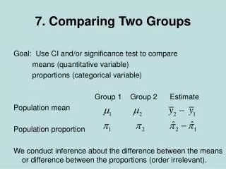
Learning Objective 3:Categorical Response Variable For a categorical response variable • Inferences compare groups in terms of their population proportions in a particular category • We can compare the groups by the difference in their population proportions: (p1 – p2)
Learning Objective 4:Example: Aspirin, the Wonder Drug • Experiment: • Subjects were 22,071 male physicians • Every other day for five years, study participants took either an aspirin or a placebo • The physicians were randomly assigned to the aspirin or to the placebo group • The study was double-blind: the physicians did not know which pill they were taking, nor did those who evaluated the results
Learning Objective 4:Example: Aspirin, the Wonder Drug Results displayed in a contingency table:
Learning Objective 4:Example: Aspirin, the Wonder Drug • What is the response variable? • The response variable is whether the subject had a heart attack, with categories ‘yes’ or ‘no’ • What are the groups to compare? • The groups to compare are: • Group 1: Physicians who took a placebo • Group 2: Physicians who took aspirin
Learning Objective 4:Example: Aspirin, the Wonder Drug • Estimate the difference between the two population parameters of interest • p1: the proportion of the population who would have a heart attack if they participated in this experiment and took the placebo • p2: the proportion of the population who would have a heart attack if they participated in this experiment and took the aspirin
Learning Objective 4:Example: Aspirin, the Wonder Drug Sample Statistics:
Learning Objective 4:Example: Aspirin, the Wonder Drug • To make an inference about the difference of population proportions, (p1 – p2), we need to learn about the variability of the sampling distribution of:
Learning Objective 5:Standard Error for Comparing Two Proportions • The difference, , is obtained from sample data • It will vary from sample to sample • This variation is the standard error of the sampling distribution of :
Learning Objective 6:Confidence Interval for the Difference Between Two Population Proportions • The z-score depends on the confidence level • This method requires: • Categorical response variable for two groups • Independent random samples for the two groups • Large enough sample sizes so that there are at least 10 “successes” and at least 10 “failures” in each group
Learning Objective 6:Confidence Interval Comparing Heart Attack Rates for Aspirin and Placebo • 95% CI:
Learning Objective 6:Confidence Interval Comparing Heart Attack Rates for Aspirin and Placebo • Since both endpoints of the confidence interval (0.005, 0.011) for (p1- p2) are positive, we infer that (p1- p2) is positive • Conclusion: The population proportion of heart attacks is larger when subjects take the placebo than when they take aspirin
Learning Objective 6:Confidence Interval Comparing Heart Attack Rates for Aspirin and Placebo • The population difference (0.005, 0.011) is small • Even though it is a small difference, it may be important in public health terms • For example, a decrease of 0.01 over a 5 year period in the proportion of people suffering heart attacks would mean 2 million fewer people having heart attacks
Learning Objective 6:Confidence Interval Comparing Heart Attack Rates for Aspirin and Placebo • The study used male doctors in the U.S • The inference applies to the U.S. population of male doctors • Before concluding that aspirin benefits a larger population, we’d want to see results of studies with more diverse groups
Learning Objective 7:Interpreting a Confidence Interval for a Difference of Proportions • Check whether 0 falls in the CI • If so, it is plausible that the population proportions are equal • If all values in the CI for (p1- p2) are positive, you can infer that (p1- p2) >0 • If all values in the CI for (p1- p2) are negative, you can infer that (p1- p2) <0 • Which group is labeled ‘1’ and which is labeled ‘2’ is arbitrary
Learning Objective 7:Interpreting a Confidence Interval for a Difference of Proportions • The magnitude of values in the confidence interval tells you how large any true difference is • If all values in the confidence interval are near 0, the true difference may be relatively small in practical terms
Learning Objective 8:Significance Tests Comparing Population Proportions 1. Assumptions: • Categorical response variable for two groups • Independent random samples
Learning Objective 8:Significance Tests Comparing Population Proportions Assumptions (continued): • Significance tests comparing proportions use the sample size guideline from confidence intervals: Each sample should have at least about 10 “successes” and 10 “failures” • Two–sided tests are robust against violations of this condition • At least 5 “successes” and 5 “failures” is adequate
Learning Objective 8:Significance Tests Comparing Population Proportions 2. Hypotheses: • The null hypothesis is the hypothesis of no difference or no effect: H0: p1=p2 The alternative hypothesis is the hypothesis of interest to the investigator Ha: p1≠p2 (two-sided test) Ha: p1<p2 (one-sided test) Ha: p1>p2 (one-sided test)
Learning Objective 8:Significance Tests Comparing Population Proportions Pooled Estimate • Under the presumption that p1= p2, we estimate the common value of p1 and p2 by the proportion of the total sample in the category of interest • This pooled estimate is calculated by combining the number of successes in the two groups and dividing by the combined sample size (n1+n2)
Learning Objective 8:Significance Tests Comparing Population Proportions 3. The test statistic is: where is the pooled estimate
Learning Objective 8:Significance Tests Comparing Population Proportions 4. P-value: Probability obtained from the standard normal table of values even more extreme than observed z test statistic 5. Conclusion: Smaller P-values give stronger evidence against H0 and supporting Ha
Learning Objective 9:Example: Is TV Watching Associated with Aggressive Behavior? • Various studies have examined a link between TV violence and aggressive behavior by those who watch a lot of TV • A study sampled 707 families in two counties in New York state and made follow-up observations over 17 years • The data shows levels of TV watching along with incidents of aggressive acts
Learning Objective 9:Example: Is TV Watching Associated with Aggressive Behavior?
Learning Objective 9:Example: Is TV Watching Associated with Aggressive Behavior? • Define Group 1 as those who watched less than 1 hour of TV per day, on the average, as teenagers • Define Group 2 as those who averaged at least 1 hour of TV per day, as teenagers • p1 = population proportion committing aggressive acts for the lower level of TV watching • p2 = population proportion committing aggressive acts for the higher level of TV watching
Learning Objective 9:Example: Is TV Watching Associated with Aggressive Behavior? • Test the Hypotheses: H0: (p1- p2) = 0 Ha: (p1- p2) ≠ 0 using a significance level of 0.05 • Test statistic:
Learning Objective 9:Example: Is TV Watching Associated with Aggressive Behavior?
Learning Objective 9:Example: Is TV Watching Associated with Aggressive Behavior? • Conclusion: Since the P-value is less than 0.05, we reject H0 • We conclude that the population proportions of aggressive acts differ for the two groups • The sample values suggest that the population proportion is higher for the higher level of TV watching
Learning Objective 9:Test of Significance: Two Proportions Summer Jobs Example • A university financial aid office polled a simple random sample of undergraduate students to study their summer employment. • Not all students were employed the previous summer. Here are the results: • Is there evidence that the proportion of male students who had summer jobs differs from the proportion of female students who had summer jobs?
Learning Objective 9:Test of Significance: Two Proportions Summer Jobs Example Hypotheses: • Null: The proportion of male students who had summer jobs is the same as the proportion of female students who had summer jobs. [H0: p1 = p2] • Alt: The proportion of male students who had summer jobs differs from the proportion of female students who had summer jobs. [Ha: p1 ≠ p2]
Learning Objective 9:Test of Significance: Two Proportions Summer Jobs Example Test Statistic: • n1 = 797 and n2 = 732 (both large, so test statistic follows a Normal distribution) • Pooled sample proportion: • Test statistic:
Learning Objective 9:Test of Significance: Two Proportions Summer Jobs Example • Hypotheses: H0: p1 = p2 Ha: p1 ≠ p2 • Test Statistic: z = 5.07 • P-value:P-value = 2P(Z > 5.07) = 0.000000396 (using a computer) • Conclusion: Since the P-value is quite small, there is very strong evidence that the proportion of male students who had summer jobs differs from that of female students.
Learning Objective 9:Test of Significance: Two Proportions Drinking and unplanned sex • In a study of binge drinking, the percent who said they had engaged in unplanned sex because of drinking was 19.2% out of 12708 in 1993 and 21.3% out of 8783 in 2001 • Is this change statistically significant at the 0.05 significance level? The P-value is 0.0002 < .05. The results are statistically significant. But are they practically significant?
Learning Objective 10:Test of Significance: Two ProportionsClass Exercise 1 • A survey of one hundred male and one hundred female high school seniors showed that thirty-five percent of the males and twenty-nine percent of the females had used marijuana previously. Does this survey indicate a difference in proportions for the population of high school seniors? Test at α=5%,
Learning Objective 10:Test of Significance: Two ProportionsClass Exercise 2 • A random sample of 500 persons were questioned regarding political affiliation and attitude toward government sponsored mandatory testing of AIDS. The results were as follows: Is there a difference in the proportions of Democrats and Republicans who are undecided regarding mandatory testing for AIDS? Test at α=5%
Chapter 10: Comparing Two Groups Section10.2: Quantitative Response: How Can We Compare Two Means?
Learning Objectives • Comparing Means • Standard Error for Comparing Two Means • Confidence Interval for the Difference between Two Population Means • Example: Nicotine – How Much More Addicted Are Smokers than Ex-Smokers? • How Can We Interpret a Confidence Interval for a Difference of Means? • Significance Tests Comparing Population Means
Learning Objective 1:Comparing Means • We can compare two groups on a quantitative response variable by comparing their means
Learning Objective 1:Example: Teenagers Hooked on Nicotine • A 30-month study: • Evaluated the degree of addiction that teenagers form to nicotine • 332 students who had used nicotine were evaluated • The response variable was constructed using a questionnaire called the Hooked on Nicotine Checklist (HONC)
Learning Objective 1:Example: Teenagers Hooked on Nicotine • The HONC score is the total number of questions to which a student answered “yes” during the study • The higher the score, the more hooked on nicotine a student is judged to be
Learning Objective 1:Example: Teenagers Hooked on Nicotine • The study considered explanatory variables, such as gender, that might be associated with the HONC score
Learning Objective 1:Example: Teenagers Hooked on Nicotine • How can we compare the sample HONC scores for females and males? • We estimate (µ1 - µ2) by ( ): 2.8 – 1.6 = 1.2 • On average, females answered “yes” to about one more question on the HONC scale than males did
Learning Objective 1:Example: Teenagers Hooked on Nicotine • To make an inference about the difference between population means, (µ1 – µ2), we need to learn about the variability of the sampling distribution of:
Learning Objective 2:Standard Error for Comparing Two Means • The difference, , is obtained from sample data. It will vary from sample to sample. • This variation is the standard error of the sampling distribution of :
Learning Objective 3:Confidence Interval for the Difference Between Two Population Means A confidence interval for m1 – m2 is: • t.025 is the critical value for a 95% confidence level from the t distribution • The degrees of freedom are calculated using software. If you are not using software, you can take df to be the smaller of (n1-1) and (n2-1) as a “safe” estimate