Tree Structured Prognostic Model for Hepatocellular Carcinoma
430 likes | 580 Vues
Tree Structured Prognostic Model for Hepatocellular Carcinoma. Taerim Lee (1) , Hyungjun Cho (2) , Hyosuck Lee (3) (1) Dept of Information Statistics Korea National Open University

Tree Structured Prognostic Model for Hepatocellular Carcinoma
E N D
Presentation Transcript
Tree Structured Prognostic Model forHepatocellular Carcinoma Taerim Lee (1) , Hyungjun Cho (2), Hyosuck Lee (3) (1) Dept of Information Statistics Korea National Open University e-mail : trlee@mail.knou.ac.kr (2) Dept. of Biostatistics University of Maryland e-mail : hyungjun@stat.wisc.edu (3) Dept. of Internal Medicine Seoul National University e-mail : hsleemd@snu.ac.kr
Outline 1. Background 2. Motivation & Purposes 3. Analytic structure of Tree Structured Model 4. Prognostic Model of Hepatocellula carcinoma 5. Remarks
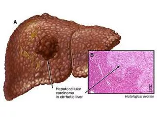
Background • Tree structured regression modeling techniques have been developed using a recursive partitioning algorithm. • There has been a strong need on the analyses of the data on the survival rate of patients with HCC who were treated with either with surgical resection or transaterial chemoembolization method.
Review of Literature 1. L. Gorden & R. Olshen & (1985)presented tree structured survival analysis in the Cancer Treatment Reports. 2. M. Segal(1988)Regression Trees for censored data 3. R.B. Davis & J.R. Anderson(1989)developed exponential survival trees using a recursive partitioning algorithm for incomplete survival data using CART in Statistics in Medicine. 4. Lynn A. Sleeper & D.P. Harrington(1990)examined a flexible survival model with Regression Splines for covariate effect in Liver Disease.
ReviewofLiterature 5.M.LeBlanc & John Crowley(1992)developed a method for obtaining tree-structured relative risk estimates for censored survival data. 6. M. LeBlanc & John Crowley(1993) reported survival trees by goodness of split in JASA. 7. H. Ahn & W.Y.Loh(1994)fitted piecewise proportional hazards models to censored survival data with bootstrapping in Biometrics. 8. D. Collett(1994)reported modeling survival data in medical search.
Review of Literature 9.W.Y. Loh & Y.S. Shih(1997)derived split selection methods for classification tree in Statistica Sinica. 10. S.H. Um et al.(1997)derived the prognostic index and define the natural stage of HCC using those index. 11. S.H. Um et al.(1998)evaluated the prognosis of HCC in relation the treatment methods. 12. S.K. Han et al.(1998)estimated the survival rate and their affecting factors in patient with HCC.
Review of Literature 14. K.M. Kim et al.(2000)studied the survival rate of patient with hepatocellular carcinoma (HCC) who were treated either with surgical resection or transarterial chemoembolization 15. K.M. Kim et al.(2000)compare the survival and quality of life in advanced non small cell lung cancer patients in Journal of Clinical Oncology. 16. H. J. Cho (2001) reported tree structured regression modeling for censored survival data.
Motivation 1. A variety of powerful modeling technique have been developed for exploring the functional form of effects for HCC. 2. To find the model related to the effects which are changing over time with covariate. 3. To obtain the tree structured prognostic models of HCC patients.
Objectives 1. To identify the effect of prognostic factors of HCC. 2. To quantify the patient characteristics that related to the survival time. 3. To explore the functional form and the relationships of the covariates. 4. To reflect the changing effects over time to the prognostic model.
Material and Method .Data : From 1993 through 1996, 186 patients with HCC in UICC T1-3NOMO and liver function of Child-Pugh class A were enrolled in SNUH. .Variables : Stratification Var: Surgical Resection group Transaterial chemoembolization group Clinical Var :sex, age, afp, viral child effect UICC. CLIP # of TACE type, tumor size, lobe, inv. Transformed variables(7) Dependent Var : prognosis(sur, sc) survivalship
CHRACTERISTIC SURGICAL TESECTION (N=91) TRANSCATHETER ARTERIAL CHEMOEMBOLIZATION (N=91) P VALUE Age-yr Mean SD 50 10 56 10 0.0002+ Male sex – no.(%) 76(84) 79(87) 0.532+ Serum alpha-fetoprotein – no.(%) 0.756+ < 400 ng/ml 58(64) 60(66) 400 ng/ml 33(36) 31(34) Viral marker-no.(%) 0.046 Hepatitis B virus 71(78) 61(67) Hepatitis C virus 4(4) 16(18) Hepatitis B and C virus 2(2) 1(1) NBNC& 13(14) 10(11) Unknown 1(1) 3(3) Table1. Pretreatment Base-Line Characteristics of the Patients
CHRACTERISTIC SURGICAL TESECTION (N=91) TRANSCATHETER ARTERIAL CHEMOEMBOLIZATION (N=91) P VALUE Okuda stage – no.(%) 0.155+ Okuda Ⅰ 91(100) 89(98) Okuda Ⅱ 0(0) 2(2) UICC T stage-no.(%) 0.003 UICC T1 17(19) 12(13) UICC T2 63(69) 49(54) UICC T3 11(12) 30(33) CLIP scoring-no.(%) 0.125 CLIP1 54(59) 39(43) CLIP2 27(30) 34(37) CLIP3 8(9) 16(18) CLIP4 2(2) 1(1) CLIP5 0(0) 1(1) Lipiodol retention pattern-no.(%) 0.063 Compact 56(62) 56(62) Non-compact 30(33) 35(38) Unknown 5(5) 0(0) Table1. Pretreatment Base-Line Characteristics of the Patients
CHRACTERISTIC SURGICAL TESECTION TRANSCATHETER ARTERIAL CHEMOEMBOLIZATION P VALUE Serum alpha-fetoprotein in total alpha-fetoprotein secretion HCC patients N=73 N=64 0.001+ No.(%) Decreased>50% 61(84) 33(52) Decreased 25-50% 7(10) 10(16) Stable0 3(4) 13(20) Increased≥25% 2(3) 8(13) Serum alpha-fetoprotein in alpha-fetoprotein secreting HCC patients with compact Lipiodol retention N=41 N=40 0.137+ No.(%) Decreased>50% 34(83) 25(63) Decreased 25-50% 4(10) 6(15) Stable0 1(2) 6(15) Increased≥25% 2(5) 3(8) Table2. Changes in afp after Initial Treatment in afp Secreating HCC
Survival Analysis - Cox regression Tree Structured Prognostic Model Analysis Comparison between survival groups
Analytic Structure of Survival Model Proportional Hazards Model (Cox 1972) Ifis the hazard rate at time y for an individual with Risk factor X, the Cox proportional hazards Model is
Fig.1 Survival Curves for HCC according to Treatment Group Median survival Resection : 59.1 months TACE : 35.5 months Variables in the Model Exp(B) CHILD 2.67 CLID 1.43 TX 0.64 EFFECT 0.54
Fig.2 Survival Curves for HCC according to Tumor Stage
Fig.3 Survival Curves for HCC according to CLIP Stage
Fig.4 Survival Curves for HCC according to Lipidol Pattern
Fig.5 Survival Curves for HCC according to Child Score
total CART X1 >a X 3>c X2 >b L D L X4 >d D L tree structured prognostic model with effective covariate : CART uses a decision tree to display how data may be classified or predicted. : automatically searches for important relationships and uncovers hidden structure even in highly complex data. Analytic Structure of Prognostic Model
39 11(0) 28(1) 147 99(0) 48(1) 124 76(0) 48(1) 23 23(0) 0(1) Sensitivity 90.0% Specificity 30.3% Total 65.6% 95 52(0) 43(1) 29 24(0) 5(1) 1. AFP 100.0 2. TAENUM 88.8 3. CHILD 61.2 4. AGE 42.2 5. TX 32.1 84 50(0) 34(1) 11 2(0) 9(1) 38 15(0) 23(1) 46 35(0) 11(1) Fig.6 Tree Structured Model based on HCC data CART 186 147(0) 39(1) AFP ≤ 8.0 1 CHILD≤5.5 0 AGE≤713 0 TAENUM≤7.5 1 TAENUM≤1.5 0 1
84 37(0) 47(1) 10 9(0) 1(1) Sensitivity 71.7% Specificity 85.4% Total 78.7% 35 22(0) 13(1) 49 15(0) 34(1) 1. TAENUM 100.0 2. AFP 87.7 3. CHILD 72.3 4. SIZE 59.4 5. INV 59.0 6. CLIP 45.5 46 12(0) 34(1) 3 3(0) 0(1) 18 8(0) 10(1) 17 14(0) 3(1) 10 7(0) 3(1) 8 7(0) 1(1) Fig.7 Tree Structured Model for TACE group of HCC data CART 94 46(0) 48(1) CHILD≤5.5 0 TAENUM≤1.5 INV≤0.5 SIZE≤3.85 0 1 0 AFP≤10.4 1 0
Sensitivity 89.1% Specificity 67.9% Total 82.6% 19 6(0) 13(1) 73 58(0) 15(1) 1. AFP 100.0 2. TAENUM 72.6 3. CHILD 31.1 4. AGE 7.7 5. TX 5.3 57 51(0) 6(1) 16 7(0) 9(1) 7 1(0) 6(1) 9 6(0) 3(1) Fig.8 Tree Structured Model based for SC group of HCC SC(Surgical Resection Group) CART 92 73(0) 19(1) AFP≤8.0 1 TAENUM≤7.5 0 AGE≤639 1 0
total FACT X1 >a X 3>c X2 >b L D L X4 >d D L tree structured prognostic model with effective covariate :FACT employs statistical hypothesis test to select a variable for splitting each node and then uses discriminant analysis to find the split point . The size of the tree is determined by a set of stopping rules Analytic Structure of Prognostic Model
total QUEST X1 >a X 3>c X2 >b L D L X4 >d D L Analytic Structure of Prognostic Model :QUESTis a new classification tree algorithm derived from the FACT method. It can be used with univariate splits or linear combination splits. Unlike FACT, QUEST uses cross-validation pruning. It distinguishes from other decision tree classifiers is that when used with univariate splits the classifier performs approximately unbiaased variable selection.
total STUDI X1 >a X 3>c X2 >b L4 L L1 X4 >d L5 L3 Analytic Structure of Prognostic Model Survival Tree with Unbiased Detection of Interaction : STUDI is a tree-structured regression modeling tool. It is easy to interpret predict survival value for new case. Missing values can easily be handled and time dependent covariates can be incorporated.
Let the survival function for a covariate Xi be Where is the cumulative baseline hazard rate. Then median survival time for and individual is defined as and the cost at a node t be is defined as Analytic Structure of Prognostic Model STUDI
Analytic Structure of Prognostic Model STUDI Modified Cox-Snell(MCS) residuals: for I=1,…,n Where is the estimator of the cumulative baseline hazard function.
Covariate Type 1. n-covariate: Ordered numerical predictor used for fitting and splitting. 2. f-covariate: Ordered numerical predictor used for fitting only. 3. s-covariate: Ordered predictor used for splitting only. 4. c-covariate: Categorical predictor for splitting only
Split Covariate Selection 1. Fit a model ton and f covariates in the node. 2. Obtain the modifiedCox-Snell residuals. 3. Perform a curvature test for each of n-s-and c-covariates. 4. Perform a interaction test for each pair of n- s-and c-covariates. 5. Select the covariate which has the smallest p-value.
Bootstrap Calibration • Bootstrap estimation of a bias correction coefficient - Let (Y*, δ*) be a bootstrap sample drawn from the elements in (Y, δ). - Fit a model to (Y*, δ*, X1, …,Xp), using only the n- and f-covariates. - Compute the p-values from the χ2 curvature and interaction tests. - Convert each p-values into an absolute normal variate z*. - For r>1, if r max {zn*, znn*} ≥ max{zs*, zc*, zss*, zcc*, zns*, znc*, zsc*}, an n covariate is selected. - Repeat the above steps over a grid of r values to estimate π(r), the probability that an n-covariate is selected. - Find r0 such that π(r0) equals the proportion of n-covariates of the total number of covariates used for spitting in the sample. Interpolate linearly if necessary.
How to select the covariate with the smallest p-value? 1. If the smallest p-value is from a curvature test -select the covariate which has the smallest p-value • 2. If the smallest p-value is from an interaction test • -for a pair of n-covariates, select the one which yields the smaller total costs of two subnodes its parent node is split by the sample median. • -for s or c covariates select the one with the smaller curvature p-value. • -between n-covariates and s or c covariate select the s or c covariate.
Unbiased covariates selection 1. Fit a medel to (Y, δ , X1…XP) using only the n and f covariates. 2. Let Z’ = max{r0Zn,r0Znn,Zs,Zc, Zss,Zcc,Zns,Znc,Zsc} select the split covariate using previous selection algorithm.
Split Points or Split Sets For an ordered covariate, use exhaustive search, it use sample median or sample quantiles. For a categorical covariate, use a shortcut algorithm given in Breiman et al. 1. Cost complexity prunning technique of CART. 2. Choice of tree pruning by a test sample or by cross-validation. Pruning
child ≤7 1 182 pafp ≤3810 2 3 23 159 Treatment = Surgery 5 4 12 147 pafp ≤78 taeeff =non-compact 8 9 80 67 tean ≤6 lobe = right 18 16 17 19 43 15 24 65 taeeff =non-compact 33 32 37 36 16 49 11 13 age ≤45.1 65 64 34 15 pafp ≤7.0 131 130 8 26 afp ≤16.0 263 262 9 17 525 524 9 8 Fig.9 Tree-Structured Survival Model for HCC
Fig.10 Scatterplot or Boxplots of the MCS Resideals
Fig.11 Survival Curves for HCC according to Node Groups
Pafp ≤5.0 1 91 2 3 34 57 Fig.12 Tree-Structured Survival Model for HCC with Surgery
Fig.13 Survival Curves for HCC with Surgery according to pafp Score
taen ≤7 1 91 pafp ≤36.0 2 3 26 65 4 5 39 25 Fig.14 Tree-Structured Survival Model for HCC with TACE
Fig.15 Survival Curves for HCC with TACE according to Node Groups
Remarks 1. The effects of prognostic factors of HCC were identified with the tree structured survival model. 2. The factors CHILD, the number of TACE treatment, AFP, PAFP level were common to all the models, the post AFP was specifically important to the survival time of surgical resection group and TACE treatment group. 3. Tree structured survivalmodel with minimum SAD provide the critical values of splitting covariates for each node.