Download

1 / 40
400 likes | 412 Vues
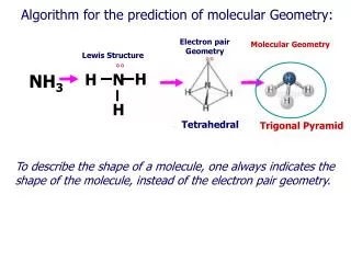
Feature selection and transduction for prediction of molecular bioactivity for drug design. Reporter: Yu Lun Kuo (D95922037) E-mail: sscc6991@gmail.com Date: April 17, 2008. Bioinformatics Vol. 19 no. 6 2003 (Pages 764-771). Abstract. Drug discovery

E N D
Feature selection and transduction for prediction of molecular bioactivity for drug design Reporter: Yu Lun Kuo (D95922037) E-mail: sscc6991@gmail.com Date: April 17, 2008 Bioinformatics Vol. 19 no. 6 2003 (Pages 764-771)
Abstract • Drug discovery • Identify characteristics that separate active (binding) compounds from inactive ones. • Two method for prediction of bioactivity • Feature selection method • Transductive method • Improvement over using only one of the techniques
Introduction (1/4) • Discovery of a new drug • Testing many small molecules for their ability to bind to the target site • The task of determining what separate the active (binding) compounds from the inactive ones
Introduction (2/4) • Design new compounds • Not only bind • But also possess certain other properties required for a drug • The task of determination can be seen in a machine learning context as one of feature selection
Introduction (3/4) • Challenging • Few positive examples • Little information is given indicating positive correlation between features and the labels • Large number of features • Selected from a huge collection of useful features • Some features are in reality uncorrelated with the labels • Different distributions • Cannot expect the data to come from a fix distribution
Introduction (4/4) • Many conventional machine learning algorithms are illequipedto deal with these • Many algorithms generalize poorly • The high dimensionality of the problem • The problem size many methods are no longer computationally feasible • Most cannot deal with training and testing data coming from different distributions
Overcome • Feature selection criterion • Called unbalanced correlation score • Take into account the unbalanced nature of the data • Simple enough to avoid overfitting • Classifier • Takes into account the different distributions in the test data compared to the training data • Induction • Transduction
Overcome • Induction • Builds a model based only on the distribution of the training data • Transduction • Also take into account the test data inputs • Combining these two techniques we obtained improved prediction accuracy
KDD Cup Competition (1/2) • We focused on a well studies data set • KDD Cup 2001 competition • Knowledge Discovery and Data Mining • One of the premier meetings of the data mining community • http://www.kdnuggets.com/datasets/kddcup.html
KDD Cup Competition (2/2) • KDD Cup 2006 • data mining for medical diagnosis, specifically identifying pulmonary embolisms from three-dimensional computed tomography data • KDD Cup 2004 • features tasks in particle physics and bioinformatics evaluated on a variety of different measures • KDD Cup 2002 • focus: bioinformatics and text mining • KDD Cup 2001 • focus: bioinformatics and drug discovery
KDD Cup 2001 (1/2) • Objective • Prediction of molecular bioactivity for drug design -- binding to Thrombin • Data • Training: 1909 cases (42 positive), 139,351 binary features • Test: 634 cases
KDD Cup 2001 (2/2) • Challenge • Highly imbalanced, high-dimensional, different distribution • Approach • Bayesian network predictive model • Data PreProcessor system • BN PowerPredictor system • BN PowerConstructor system
Data Set (1/3) • Provided by DuPont Pharmaceuticals • Drug binds to a target site on thrombin, a key receptor in blood clotting • Each example has a fixed length vector of 139,351 binary features in {0, 1} • Which describe three-dimensional properties of the molecule
Data Set (2/3) • Positive examples are labeled +1 • Negative examples are labeled -1 • In the training set • 1909 examples, 42 of which bind (rather unbalanced, positive is 2.2%) • In the test set • 634 additional compounds
Data Set (3/3) • An important characteristic of the data • Very few of the feature entries are non-zero (0.68% of the 1,909 X 139,351 training matrix)
System Assessment • Performance is evaluated according to a weighted accuracy criterion • The score of an estimate y’ of the labels y • Complete success is a score of 1 • Multiply this score by 100 as the percentage weighted success rate
Methodology • Predict the labels on the test set by using a machine learning algorithm • The positively and negatively labeled training examples are split randomly into n groups • For n-fold cross validation such that as close to 1/n of the positively labeled examples are present in each group as possible • Called balanced cross validation • As few positive examples
Methodology • The method is • Trained on n-1 of groups • Tested on the remaining group • Repeated n times (different group for testing) • Final score: mean of the n scores
Feature Selection (1/2) • Called the unbalanced correlation score • fj: the score of feature j • X: training data as a matrix X where columns are features and examples are rows • Take λ very large in order to select features which have non-zero entries (λ ≧3)
Feature Selection (2/2) • This score is an attempt to encode prior information that • The data is unbalanced • Large number of features • Only positive correlations are likely to be useful
Justification • Justify the unbalanced correlation score using methods of information theory • Entropy: higher non-regular • Pi: the probability of appearance of event i
Entropy • The probability of random appearance of a feature with an unbalanced score of N=Np-Nn • Np= number of one entries associated to +1 • Nn= number of one entries associated to -1 • Tp= total number of positive labels in training set • Tn= total number of negative labels in training set
Entropy • Need to compute the probability that a certain N might occur randomly • Finally, compute the entropy for each feature
Entropy and unbalanced score • The entropy and unbalanced score will not reach the same feature • Because the unbalanced correlation score will no select samples with low negative • In this particular problem • Reach a similar ranking of the features • Due to the unbalanced nature of the data
Entropy and unbalanced score • The first 6 features for both scores • 5 out of 6 are the same ones • For 16 features, 12 coincide • Pay more attention to positive correlations
Multivariate unbalanced correlation • The feature selection algorithm described so far is univariate • Reduces the chance of overfitting • Between the inputs and targets are too complex this assumption may be to restrictive • We extend our criterion to assign a rank to a subset of feature • Rather than just a single feature
Multivariate unbalanced correlation • By computing the logical OR of the subset of features S (as they are binary)
Fisher Score • μ(+): the mean of the feature values for positive • μ(-): the mean of the feature values for negative • σ(+): standard deviations • σ(-): standard deviations
In each case, the algorithms are evaluated for different numbers of features d • The range d = 1, …, 40 • Choose a small number of features in order to render interpretability of the decision function • It is anticipated that a large number of features are noisy and should not be selected
Classification algorithms (Inductive) • The task may not simply be just to identify relevant characteristics via feature selection • But also to provide a prediction system • Simplest of classifiers • We call this a logical OR classifier
Comparison Techniques • We compared a number of rather more sophisticated classification • Support vector machines (SVM) • SVM* • Make a search over all possible values of the threshold parameter in the linear model after training • K-nearest neighbors (K-NN) • K-NN* (parameter γ) • C4.5 (decision tree learner)
Transductive Inference • One is given labeled data from which builds a general model • Then applies this model to classify previously unseen (test) data • Takes into account not only the given (labeled) training set but also unlabeled data • That one wishes to classify
Transductive Inference • Different models can be built • Trying to classify different test sets • Even if the training set is the same in all cases • It is this characteristic which help to solve problem 3 • The data we are given has different distribution in the training and test sets
Transductive Inference • Transduction is not useful in all tasks • In drug discovery in particular we believe it is useful • Developers often have access to huge databases of compounds • Compounds are often generated using virtual Combinatorial Chemistry • Compound descriptors can be computed even though the compounds have not been synthesized yet
Transductive Inference • Drug discovery is an iterative process • Machine learning method is to help choose the next test set • Step in a two-step candidate selection procedure • After candidate test set has been produced • Its result is the final test set
Results (with unbalanced correlation score) • C4.5 gave only 50% success rate for all The tansductive algorithm is consistently selecting more relevant features than the inductive one the Fisher score
Further Results • We also tested some more sophisticated multivariate feature selection methods • Not as good as using the unbalanced criterion score • Using non-linear SVMs • Not improve results (50% success) • SVMs as a base classifier for our transduction • Improvement over using SVMs
Further Results • Also tried training the classifiers with larger numbers of features • Inductive methods • failed to learn anything after 200 features • Transductive methods • Exhibit generalization behavior up to 1000 features • (TRANS-Orcub:58% success with d=1000,77% with d=200) • KDD champion • Success rate 68.4% (7% of entrants higher than 60%)