A Novel approach to solving large-scale linear systems
300 likes | 432 Vues
This document presents a novel method for solving large-scale linear systems, addressing the limitations of traditional approaches like Gaussian elimination and LU decomposition, which can have high computational complexity. It revisits Cramer’s rule and introduces matrix condensation techniques that allow for improved parallel processing capabilities. Scientific applications across finance, biology, and physics are discussed, alongside challenges in real-time calculations for electric utilities, indicating a significant evolution in computational strategies for handling complex linear equations.

A Novel approach to solving large-scale linear systems
E N D
Presentation Transcript
Gabriel cramer (1704-1752) A Novel approach to solving large-scale linear systems Ken Habgood, ItamarArel Department of Electrical Engineering & Computer Science April 3, 2009
Outline • Problem statement and motivation • Novel approach • Revisiting Cramer’s rule • Matrix condensation • Illustration of the proposed scheme • Implementation results • Challenges ahead
Solving large-scale linear systems • Many scientific applications • Computer models in finance, biology, physics • Real-time load flow calculations for electric utilities • Short-circuit fault, economic analysis • Consumer generation on the electric grid may soon require real-time calculations (hybrid cars, solar panels)
Why try to improve? • We want parallel processing for speed • Current schemes use Gaussian elimination • Mainstream approach: LU decomposition • O(N3) computational complexity, O(N2) parallelizable • If you had N2 processors O(N) time • So far so good … • The “catch”: Irregular communication patterns for load balancing across processing nodes
Cramer’s rule revisited 5 • The solution to a linear system Ax = b is given by • xi = |Ai(b)|/|A| • where Ai(b) denotes A with its ith column replaced by b e b f d ax + by = e cx + dy = f x = a b c d • O(N!) computational complexity
Chio’s matrix condensation 6 a1,1 a1,j ai,1 ai,j • Let D denote the matrix obtained by replacing each element ai,j by |D| • a1,1 cannot be 0 • If a1,1 is 1 then a1,1–(n-2) =1 Then |A| = a1,1n-2 Matrix A a1 b1 a2 b2 a1 c1 a2 c2 a1 b1 c1 a2 b2 c2 a3 b3 c3 b2’ c2’ b3’ c3’ = a1–(n-2) = a1–(n-2) a1 b1 a3 b3 a1 c1 a3 c3 • Recursive determinant calculation • O(N3) computational complexity
Highlights of the approach 7 • Chio’s condensation combined with Cramer’s rule results in O(N4) • Goal to remain at O(N3) • Retain attractive parallel processing potential • Solution: clever bookkeeping to reduce computations • “Mirror” matrix before applying condensation • Each matrix solves for half of the unknowns • Condense each until matrix size matches the number of unknowns • Mirror the matrices again
Mirroring the matrix 3 3 -1 -1 4 4 3 3 2 2 3 3 -4 -4 4 4 -5 -5 -4 3 3 -1 -1 2 2 -2 -2 4 4 -2 -2 -3 -3 -2 -2 -2 -2 4 2 2 -5 -5 3 3 3 3 -5 -5 0 0 -5 -5 -2 -2 0 0 0 1 1 -1 -1 4 4 1 1 -2 -2 2 2 0 0 0 0 1 1 1 2 2 0 0 -4 -4 -1 -1 4 4 -5 -5 2 2 -4 -4 -1 -1 -4 -5 -5 -4 -4 -4 -4 4 4 -5 -5 -3 -3 0 0 -5 -5 0 0 -5 0 0 -4 -4 0 0 0 0 3 3 4 4 -3 -3 -2 -2 0 0 4 4 4 -3 -3 -1 -1 -5 -5 1 1 -2 -2 -4 -4 -1 -1 -1 -1 0 0 0 0 0 2 2 2 2 -1 -1 2 2 4 4 -5 -5 2 2 0 9 unknowns to solve for
Mirroring the matrix (cont’) 3 -1 4 3 2 3 -4 4 -5 -4 -4 5 -4 4 -3 2 3 4 -1 3 3 -1 2 -2 4 -2 -3 -2 -2 4 4 2 2 3 2 4 -2 2 -1 3 2 -5 3 3 -5 0 -5 -2 0 0 0 0 2 5 0 -5 3 3 -5 2 1 -1 4 1 -2 2 0 0 1 1 1 -1 0 0 -2 -2 1 4 -1 1 2 0 -4 -1 4 -5 2 -4 -1 -4 -4 1 4 -2 5 4 -1 -4 0 2 -5 -4 -4 4 -5 -3 0 -5 0 -5 -5 0 5 0 3 -5 4 -4 -4 -5 0 -4 0 0 3 4 -3 -2 0 4 4 0 2 3 -4 3 0 0 -4 0 4 -3 -1 -5 1 -2 -4 -1 -1 0 0 1 1 4 2 1 -5 -1 -3 4 0 0 2 2 -1 2 4 -5 2 0 0 -2 5 -4 -2 -1 2 2 0 0
Mirroring the matrix (cont’) 3 -1 4 3 2 3 -4 4 -5 -4 5 -4 4 -3 2 3 4 -1 3 -4 3 -1 2 -2 4 -2 -3 -2 -2 4 2 2 3 2 4 -2 2 -1 3 4 2 -5 3 3 -5 0 -5 -2 0 0 0 2 5 0 -5 3 3 -5 2 0 1 -1 4 1 -2 2 0 0 1 1 -1 0 0 -2 -2 1 4 -1 1 1 2 0 -4 -1 4 -5 2 -4 -1 -4 1 4 -2 5 4 -1 -4 0 2 -4 -5 -4 -4 4 -5 -3 0 -5 0 -5 0 5 0 3 -5 4 -4 -4 -5 -5 0 -4 0 0 3 4 -3 -2 0 4 0 2 3 -4 3 0 0 -4 0 4 4 -3 -1 -5 1 -2 -4 -1 -1 0 1 1 4 2 1 -5 -1 -3 4 0 0 0 2 2 -1 2 4 -5 2 0 -2 5 -4 -2 -1 2 2 0 0 0 4 unknowns to solve for 5 unknowns to solve for
Mirroring the matrix (cont’) 3 -1 4 3 2 3 -4 4 -5 -4 5 -4 4 -3 2 3 4 -1 3 -4 3 -1 2 -2 4 -2 -3 -2 -2 4 2 2 3 2 4 -2 2 -1 3 4 2 -5 3 3 -5 0 -5 -2 0 0 0 2 5 0 -5 3 3 -5 2 0 1 -1 4 1 -2 2 0 0 1 1 -1 0 0 -2 -2 1 4 -1 1 1 2 0 -4 -1 4 -5 2 -4 -1 -4 1 4 -2 5 4 -1 -4 0 2 -4 -5 -4 -4 4 -5 -3 0 -5 0 -5 0 5 0 3 -5 4 -4 -4 -5 -5 0 -4 0 0 3 4 -3 -2 0 4 0 2 3 -4 3 0 0 -4 0 4 4 -3 -1 -5 1 -2 -4 -1 -1 0 1 1 4 2 1 -5 -1 -3 4 0 0 0 2 2 -1 2 4 -5 2 0 -2 5 -4 -2 -1 2 2 0 0 0 4 unknowns to solve for 5 unknowns to solve for
Chio’s matrix condensation 3 -1 4 3 2 3 -4 4 -5 -4 3 -1 2 -2 4 -2 -3 -2 -2 4 2 -5 3 3 -5 0 -5 -2 0 0 1 -1 4 1 -2 2 0 0 1 1 2 0 -4 -1 4 -5 2 -4 -1 -4 -5 -4 -4 4 -5 -3 0 -5 0 -5 0 -4 0 0 3 4 -3 -2 0 4 4 -3 -1 -5 1 -2 -4 -1 -1 0 0 0 2 2 -1 2 4 -5 2 0
Chio’s matrix condensation (cont’) = 0 3 -1 4 3 2 3 -4 4 -5 -4 3 -1 2 -2 4 -2 -3 -2 -2 4 2 -5 3 3 -5 0 -5 -2 0 0 1 -1 4 1 -2 2 0 0 1 1 2 0 -4 -1 4 -5 2 -4 -1 -4 -5 -4 -4 4 -5 -3 0 -5 0 -5 0 -4 0 0 3 4 -3 -2 0 4 4 -3 -1 -5 1 -2 -4 -1 -1 0 0 0 2 2 -1 2 4 -5 2 0
Chio’s matrix condensation (cont’) 3 -1 = -6 3 4 3 2 3 -4 4 -5 -4 0 2 -2 4 -2 -3 -2 -2 4 2 -5 3 3 -5 0 -5 -2 0 0 1 -1 4 1 -2 2 0 0 1 1 2 0 -4 -1 4 -5 2 -4 -1 -4 -5 -4 -4 4 -5 -3 0 -5 0 -5 0 -4 0 0 3 4 -3 -2 0 4 4 -3 -1 -5 1 -2 -4 -1 -1 0 0 0 2 2 -1 2 4 -5 2 0
Chio’s matrix condensation (cont’) 3 = 24 3 -4 -1 4 3 2 3 -4 4 -5 0 -6 -15 6 -15 3 -18 9 4 2 -5 3 3 -5 0 -5 -2 0 0 1 -1 4 1 -2 2 0 0 1 1 2 0 -4 -1 4 -5 2 -4 -1 -4 -5 -4 -4 4 -5 -3 0 -5 0 -5 0 -4 0 0 3 4 -3 -2 0 4 4 -3 -1 -5 1 -2 -4 -1 -1 0 0 0 2 2 -1 2 4 -5 2 0
Chio’s matrix condensation (cont’) 3 4 = -13 3 -1 4 3 2 3 -4 4 -5 0 -6 -15 6 -15 3 -18 9 24 2 -5 3 3 -5 0 -5 -2 0 0 1 -1 4 1 -2 2 0 0 1 1 2 0 -4 -1 4 -5 2 -4 -1 -4 -5 -4 -4 4 -5 -3 0 -5 0 -5 0 -4 0 0 3 4 -3 -2 0 4 4 -3 -1 -5 1 -2 -4 -1 -1 0 0 0 2 2 -1 2 4 -5 2 0
Chio’s matrix condensation (cont’) -1 3 = 2 4 3 2 3 -4 4 -5 3 0 -6 -15 6 3 -18 9 24 -15 -13 1 3 -19 -6 -7 -14 10 8 1 -2 8 0 -8 3 4 -4 8 7 2 2 -20 -9 8 -21 14 -20 7 -4 -5 -17 8 27 -5 6 -20 5 -25 -35 0 -12 0 0 9 12 -9 -6 0 12 4 -5 -19 -27 -5 -18 4 -19 17 16 0 0 6 6 -3 6 12 -15 6 0
Chio’s matrix condensation (cont’) The value in the a1,1 position cannot be zero 0 -6 -15 6 3 -18 9 24 -15 -13 1 3 -19 -6 -7 -14 10 8 -2 8 0 -8 3 4 -4 8 7 2 -20 -9 8 -21 14 -20 7 -4 -17 8 27 -5 6 -20 5 -25 -35 -12 0 0 9 12 -9 -6 0 12 -5 -19 -27 -5 -18 4 -19 17 16 0 6 6 -3 6 12 -15 6 0
Mirroring the matrix -3 7 -5 5 -2 -1 9 -3 -2 -2 -7 -2 9 7 -1 3 -4 0 -5 6 2 6 -1 -9 1 -1 4 -7 2 2
Mirroring the matrix (cont’) -3 7 -5 5 -2 -3 -1 7 -5 5 -2 -1 9 -3 -2 -2 -7 -2 9 -3 -2 -2 -7 -2 9 7 -1 3 3 -4 0 9 7 -1 -4 0 -5 6 2 6 1 1 -9 -9 -5 6 2 6 1 -1 4 -7 2 2 1 -1 4 -7 2 2
Chio’s matrix condensation -5 5 7 -1 -3 -2 -3 7 -5 5 -2 -1 -3 7 2 -2 9 -2 9 -3 -2 -2 -7 -2 -6 19 -17 8 -8 -3 7 4 -1 9 0 9 7 -1 3 -4 0 4 20 -12 11 -6 -1 6 -9 -6 2 -5 -5 6 2 6 1 -9 8 -10 14 -7 -6 -1 -2 7 4 1 2 1 -1 4 -7 2 2 -1 6 -9 4 1 3 unknowns to solve for 2 unknowns to solve for
Applying Cramer’s rule -6 -6 19 19 -17 -17 8 8 -8 -8 4 4 20 20 -12 -12 11 11 -6 -6 8 8 -10 -10 14 14 -7 -7 -6 -6 -1 -1 6 6 -9 -9 4 4 1 1
Applying Cramer’s rule -6 19 -17 8 -8 4 20 -12 11 -6 7728 = 8 -10 14 -7 -6 -1 6 -9 4 1 -6 19 -17 8 3 Answer for x9 = 4 20 -12 11 2688 = 8 -10 14 -7 -1 6 -9 4
Applying Cramer’s rule -6 19 -17 -8 8 4 20 -12 -6 11 180 = 8 -10 14 -6 -7 -1 6 -9 1 4 -6 19 -17 8 0.07 Answer for x8 = 4 20 -12 11 2688 = 8 -10 14 -7 -1 6 -9 4
Overview of data flow structure 25 Mirroring of the matrix keeps an O(N3) algorithm. 24 variables Original Matrix (N) 12 variables 12 variables Original Matrix (N) Original Matrix Mirror (N) Chio’s condensation Chio’s condensation (N/2) (N/2) 6 variables 6 variables 6 variables 6 variables (N/2) Image (N/2) Image (N/2) (N/2) (N/4)Image (N/4)Image (N/4) (N/4) (N/4) (N/4) I (N/4) (N/4) (N/4) I (N/4) (N/4) I (N/4) I 3 x 3 3 x 3 3 x 3 3 x 3 3 x 3 3 x 3 3 x 3 3 x 3
Parallel computations Similar to LU-decomposition (Access by rows) Broadcast communication only Send-ahead on lead row values 26 • Mirroring provides an advantage • Algorithm mirrors as matrix reduces in size • Load naturally redistributed among processors • LU-decomposition needs blocking and interleaving to avoid idle processors, leads to complex communication patterns (overhead) Figure 9.2: Parallel Scientific Computing in C++ and MPI. George Em Karniadakis and Robert M. Kirby II
Paradigm shift – key points • Apply Cramer’s rule • Employ matrix condensation for efficient determinant calculations • Highly parallel O(N3) process • Clever bookkeeping to re-use information • Final result O(N3) comp. with O(N2) comm. • Key advantage: regular communication patterns with low comm overhead and balanced processing load
Implementation results • Trial platform • Single-core Pentium M @ 1.5 GHz • 64 KB L1 cache, 1 MB L2 cache • Coded in C with SSE used for core function (Chio’s condensation) • Memory access optimized using cache blocking • Double precision variables and calculations • Result: ~2.4x slower than Matlab (consistently)
Challenges ahead • Further code improvement/optimization • Current L2 miss rate is high • Precision improvement • Parallel implementation • GPU implementation • Distributed architecture implementation • Sparse matrix optimization • Other linear algebra applications (e.g. matrix inversion)