Accuracy Assessment
490 likes | 600 Vues
Accuracy Assessment. Chapter 14. Significance. Accuracy of information is surprisingly difficult to address We may define accuracy, in a working sense, as the degree (often as a percentage) of correspondence between observation and reality .

Accuracy Assessment
E N D
Presentation Transcript
Accuracy Assessment Chapter 14
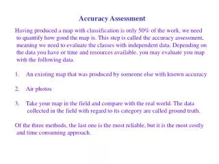
Significance • Accuracy of information is surprisingly difficult to address • We may define accuracy, in a working sense, as the degree (often as a percentage) of correspondence between observation and reality. • We usually judge accuracy against existing maps, large scale aerial photos, or field checks.
Significance • We can pose two fundamental questions about accuracy: • Is each category in a classification really present at the points specified on a map? • Are the boundaries separating categories valid as located?
Various types of errors diminish the accuracy of feature identification and category distribution. • We make most of the errors either in measuring or in sampling. • Three types of errors dominate
Data Acquisition Errors: • These include sensor performance, stability of the platform, and conditions of viewing. • Reduce or compensate for them by making systematic corrections (e.g., by calibrating detector response with on-board light sources generating known radiances). • Make corrections using ancillary data such as known atmospheric conditions, during the initial processing of the raw data.
Data Processing Errors: • An example is misregistration of equivalent pixels in the different bands of the Landsat Thematic Mapper. • Geometric correction should keep the mismatch to a displacement to one pixel. • Under ideal conditions, and with as many as 25 ground control points (GCP) spread around a scene, we can realize this goal. • Misregistrations of several pixels significantly compromise accuracy.
Scene-dependent Errors: One such error relates to how we define and establish the class, which, in turn, is sensitive to the resolution of the observing system and the reference map or photo. Mixed pixels fall into this category.
Ancillary data • An often overlooked point about maps as reference standards is their intrinsic or absolute accuracy. • Maps require an independent frame of reference to establish their own validity. • For centuries, most maps were constructed without regard to assessment of their inherent accuracy.
Ancillary data • In recent years, some maps come with a statement of confidence level. • The U.S. Geological Survey has reported results of accuracy assessments of the 1:250,000 and 1:1,000,000 land use maps of Level 1 classifications, based on aerial photos, that meets the 85% accuracy criterion at the 95% confidence level.
Rand McNally map Landsat ETM+ image
Obtainable Accuracy • Level of accuracy obtainable depends on diverse factors, such as • the suitability of training sites, • the size, shape, distribution, and frequency of occurrence of individual areas assigned to each class • which together determine the degree to which pixels are mixed,
Obtainable Accuracy • Sensor performance and resolution • The methods involved in classifying (visual photointerpreting versus computer-aided statistical classifying). • A quantitative measure of the mutual role of improved spatial resolution and size of target on decreasing errors appears in this plot:
The dramatic improvement in reducing errors ensues for resolutions of 30 m (98 ft) or better. • This relates, in part, to the nature of the target classes. • Coarse resolution is ineffective in distinguishing crop types, but high resolution (< 20 m) adds little in recognizing these other than perhaps identifying species
As the size of crop fields increases, the error decreases further. • The anomalous trend for forests (maximum error at high resolution) may be the consequence of the dictum: "Can't see the forest for the trees". • Here high resolution begins to display individual species and breaks in the canopy that can confuse the integrity of the class "forest". • Two opposing trends influence the behavior of these error curves: • 1) statistical variance of the spectral response values decreases whereas • 2) the proportion of mixed pixels increases with poorer resolution.
Accuracy and Precision • Accuracy is the “correctness” • Precision is the detail • We may increase accuracy by decreasing precision • If we define something as “forest” it could include pine, broadleaf, scrub, etc.
Significance • Why is it important • Legal standing of maps and reports • Operational usefulness • Validity as basis of scientific research • Should be evaluated through a well-defined, quantitative process • This needs to be supported by independent evidence
Sources of error • Errors is exist in any classification • Misidentification • Excessive generalization • Misregistration • Etc • Simplest error may be misassignment of informational categories to spectral categories
Sources of error • Most errors probably caused by complex factors • Mixed pixels • A simple landscape with large uniform parcels is the easiest to classify
Sources of error • Important Landscape Variables • Parcel size • Variation in parcel size • Parcel type • Number of types • Arrangement of different types • Number of parcels per type • Shapes of parcels • Radiometric and spectral contrasts
Sources of error • Errors change from region to region and date to date
Error characteristics • Classification error – assignment of a pixel in one category to another category • Errors are not randomly distributed across the image • Errors are not random to various categories • Tend to show clumped distribution on space • Errors may have spatial correlation to parcels • Occur at edges or in the interior
Map Accuracy Measurement • The task is to compare a map prepared from RS data, with another map (reference map) created from different source material. • The reference map is assumed to be accurate • If seasonal changes are important, reference should also reflect this
Map Accuracy Measurement • Both maps must register • Both maps must use the same classifications • Both maps must be mapped at same level of detail
Map Accuracy Measurement • Simplest comparison is total area of each class • Called non-site-specific accuracy • Imperfect because underestimation in one are can be compensated by overestimation in another • Called inventory error
Map Accuracy Measurement • Site specific accuracy is based on detailed assessment between the two maps • In most cases pixels are the unit of comparison • Known as classification error • This is misidentification of pixels • There may also be boundary errors
Error Matrix • In the evaluation of classification errors, a classification error matrix is typically formed. • This matrix is sometimes called confusion matrix or contingency table. • In this table, classification is given as rows and verification (ground truth) is given as columns for each sample point.
Error Matrix • The diagonal elements in this matrix indicate numbers of sample for which the classification results agree with the reference data. • Off diagonal elements in each row present the numbers of sample that has been misclassified by the classifier, • i.e., the classifier is committing a label to those samples which actually belong to other labels. The misclassification error is called commission error. • The off-diagonal elements in each column are those samples being omitted by the classifier. • Therefore, the misclassification error is also called omission error.
Error Matrix • The most common error estimate is the overall accuracy • From the example of confusion matrix, we can obtain ω = (28 + 15 + 20)/100 = 63%.
Error Matrix • More specific measures are needed because the overall accuracy does not indicate how the accuracy is distributed across the individual categories. • The categories could, and frequently do, exhibit drastically differing accuracies but overall accuracy method considers these categories as having equivalent or similar accuracies.
Error Matrix • From the confusion matrix, it can be seen that at least two methods can be used to determine individual category accuracies. • (1) The ratio between the number of correctly classified and the row total • the user's accuracy - because users are concerned about what percentage of the classes has been correctly classified. • (2) The ratio between the number of correctly classified and the column total • is called the producer's accuracy.
Error Matrix • A more appropriate way of presenting the individual classification accuracies. • Commission error = 1 - user's accuracy • Omission error = 1 - producer's accuracy Overall Accuracy Consumer’s Accuracy Producer’s Accuracy
Producers accuracy = 1- 0.067=0.933 • 0r 93.3 % • Consumers Accuracy = 1-0.51=0.49 • Or 49%
The Kappa coefficient • The Kappa coefficient (K) measures the relationship between beyond chance agreement and expected disagreement. • This measure uses all elements in the matrix and not just the diagonal ones. • The estimate of Kappa is the proportion of agreement after chance agreement is removed from consideration:
The Kappa coefficient • = (po - pc)/(1 - pc) = (obs – exp)/(1-exp) • po = proportion of units which agree, =Spii = overall accuracy • pc = proportion of units for expected chance agreement =Spi+ p+i • pij = eij/NT • pi+ = row subtotal of pij for row i • p+i = column subtotal of pij for column i
Error Matrix Grand Total = 100, Total correct = 63, Observed correct = 63/100 = 0.63
Pi+ = 0.3 x 0.57 = .171, 0.3 x 0.21 = .063, 0.4 x 0.22 = 0.88 Pc = Exp correct = 0.171 + 0.063 + 0.088 = 0.322 Po = Obs correct = 0.28 + 0.15 + 0.2 = 0.63 (Overall Accuracy)
Kappa Coefficient • One of the advantages of using this method is that we can statistically compare two classification products. • For example, two classification maps can be made using different algorithms and we can use the same reference data to verify them. • Two s can be derived, 1, 2. For each , the variance can also be calculated.
Another Way • The following shows an alternative way to do the error matrix • Errors of Omission and Commission are both calculated from the row totals in this technique