Download
1 / 27
270 likes | 391 Vues
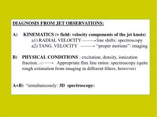
DIAGNOSIS FROM JET OBSERVATIONS: KINEMATICS (v field: velocity components of the jet knots) a1) RADIAL VELOCITY line shifts: spectroscopy a2) TANG. VELOCITY “proper motions”: imaging

E N D
DIAGNOSIS FROM JET OBSERVATIONS: • KINEMATICS (v field: velocity components of the jet knots) • a1) RADIAL VELOCITY line shifts: spectroscopy • a2) TANG. VELOCITY “proper motions”: imaging • PHYSICAL CONDITIONS : excitation, density, ionization fraction…. Appropriate flux line ratios: spectroscopy (quite rough estimation from imaging in different filters, however) • A+B) “simultaneously: 3D spectroscopy:
IMAGING: WHAT CAN BE DERIVED FROM? Obtain images through “narrow-band” ( FWHM ~ 50 A) filters of the HHs field: HHs emission is mainly “pure line emission” (except near the source) use filters centered on brighter characteristic jet emission lines, eg, Optical: Ha, [SII] red doublet, [OIII] (less used: extinction and excitation conditions..) Infrared: [FeII], H2 Morphology: “history” of the mass-ejection jet/environment interaction (indirect) evidence on the nature of the jet source and ejection mechanisms spatial distribution of the physical conditions through the jet… Kinematics: VT, from “proper motions”
NARROW-BAND (OPTICAL) FILTERS Commonly used for HHs (from NOT webpage): “Ha” filter [SII] “red” filter ([SII] 6717, 6731 A) (6563+part of [NII] 6584 A)
Narrow-band (NIR) filters Commonly used for HHs imaging (from ING webpage) H2 2.12 mm (K band) [FeII] 1.64 mm (H band)
KINEMATICS:TANGENTIAL VELOCITY OF THE KNOTS (VT) Knots of the jets appear “displaced” relative to the field stars when images obtained at different epochs are compared. By measuring these “displacements” between two epochs, the VT can be obtained (for a knwon distance). HST high-spatial resolution images have shown the “displacement” of the knot structures with time, with high degree of detai,l in several wellknown HH jets.
HH 111 HST images from (Hartigan et al..)
Bally et al. (2002), AJ,123,2627. CS * HH 1 HH 2 HST (1997) N
Bally et al. (2002), AJ,123,2627. HST (1994); proper motions after 5 yrs.
Bally et al. (2002), AJ,123,2627. HST (1994); proper motions in 5 yrs.
HH 47 Proper motions Arrow:: displacement in 30 yrs HH 47
Proper-motions from ground-based images: two examples Summary: 1) Obtain several images of the jet field, with appropriate time spacing, through narrow-band filters covering emission from [SII] or Ha (strong emission lines at visible wavelengths). 2) Convert all the images on to a common reference system, using positions of field stars. . Highly recommended: reference stars, well distributed around jet (not always possible, extinction!) . Different images from different instruments: care with their spatial scale! 3) Identify each of the knots of the jet in all the images Care! Some structures may have changed with time 4) Evaluate the (spatial) displacement of each of the knots, with respect to the (fixed) reference star system, during the time elapsed between two images n pixel/yr n arcsec/yr : PROPER MOTION (+ distance) VT (kms-1)
Ex. 1: HH 110 . In Orion B cloud complex (d~450pc) . It shows “peculiarities, eg, : rather chaotic morphology exciting source, unknown originated by deflection of HH 270 that collides with a high-density clump (see later) Reipurt & Bally (90 ´s)
HH 270 HH 110 HH 110 Sepúlveda et al., 2011, AA, 527, 41 [SII] image, 2.5m INT- 1993
HH 110 Knot identification ~4 ARCMIN N [SII] image, 2.6m NOT, 2002
HH 110 knot A 12/1993 10/2002 12/1987 López et al. 2005, A&A, 432,567 Displacement of knot A from 1987 to 2002 (after convert all images on to a common reference system).
Displacement obtained for the HH 110 knot, using images from three epochs Knot M 2002 1993 1987
HH 110: Proper motions obtained from a time baseline ~ 15 yr; for a distance ~ 450pc VT
Ex 2 HH 30 Mundt et al. A&A, 232, 37 (1990) HST archive In L1551, TMC (d~140pc) Prototypical jet/disk system. Jet/counterjet structure. “wiggling morphology”. Exciting source, “hidden” (invisible at optical/ir wavelengths)
HH 30: [SII] image, 2.6m NOT, 1998 Anglada et al., AJ,133,2799
Displacements of the jet knots of HH 30 Anglada et al. 2007, AJ,133,2799
Proper motions of the jet knots of HH 30 Anglada et al. 2007, AJ,133,2799
HH 30 [SII] image, 4.2m WHT, 2010
Displacements of the knots of the HH 30 jet/counterjet system counterjet jet with a longer time baseline: Appreciable different kinematic behaviour jet/counterjet Estalella et al, 2012,AJ,144,61
HH 30 jet/counterjet proper motions Estalella et al, 2012,AJ,144,61