Download
1 / 35
370 likes | 731 Vues
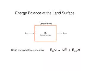
Control volume. E in. IE (internal energy). E out. E in D t = D IE + E out D t. Basic energy balance equation:. Energy Balance at the Land Surface. Energy Balance for a Single Land Surface Slab, Without Snow. S w i + L w i = S w h + L w h + H + l E + C p D T + miscellaneous.

E N D
Control volume Ein IE (internal energy) Eout EinDt = DIE + EoutDt Basic energy balance equation: Energy Balance at the Land Surface
Energy Balance for a Single Land Surface Slab, Without Snow Swi + Lwi = Swh + Lwh + H +lE + CpDT + miscellaneous Terms on LHS come from the climate model. Strongly dependent on cloudiness, water vapor, etc. Terms on RHS come are determined by the land surface model. Sw Sw Lw Lw H lE T where Swi = Incoming shortwave radiation Lwi = Downward longwave radiation Swh = Reflected shortwave radiation Lwh = Upward longwave radiation H = Sensible heat flux l = latent heat of vaporization E = Evaporation rate Cp = Heat capacity of surface slab DT = Change in slab’s temperature, over the time step miscellaneous = energy associated with soil water freezing, plant chemical energy, heat content of precipitation, etc.
Sw Sw Lw Lw H lE Note: same symbols are used, but values will be different. Internal energy T1 G12 T2 T3 Energy balance in snowpack Sw Sw Lw Lw H lsE Internal energy Tsnow lmM GS1 T1 G12 T1 Internal energy T2 G23 T3 Other energy balances can also be considered. For example: Energy balance of a vegetation canopy Energy balance in a surface layer Sw Sw Lw Lw H lE Tc Sw Sw Lw Lw H H G12 = heat flux between soil layers 1 and 2 Energy balance in a subsurface layer lm= latent heat of melting ls= latent heat of sublimation M = snowmelt rate GS1 = heat flux between bottom of pack and soil layer 1
Sw Sw Lw Lw H lE Tc Sw Sw Lw Lw H H In practice, several energy balance calculations may be combined into a single “model” Sw Sw Lw Lw H lsE lE Tsnow lmM GS1 T1 G12 T2 G23 T3 The trick is to keep the fluxes between the “control volumes” consistent. If the energy balance calculation for the snowpack includes a flux GS1 from the bottom of the pack to the ground, then the energy balance for the top soil layer must include an input flux of GS1. In the above example, a total of five energy balances are computed: one for the canopy, one for the snowpack, and one for each of three soil layers. Note that some models may include additional soil layers or may divide the snowpack itself into layers, each with its own energy balance.
Reflected Shortwave Radiation # bands # bands Assume: Sw = S Swdirect, band b + S Swdiffuse, band b b=1 b=1 reflectance for spectral band Compute: Sw = S Sw direct, band b a direct, band b + S Sw diffuse, band b a diffuse, band b # bands b=1 # bands b=1 Simplest description: consider only one band (the whole spectrum) and don’t differentiate between diffuse and direct components: Sw = Sw a Typical albedoes (from Houghton): sand .18-.28 grassland .16-.20 green crops .15-.25 forests .14-.20 dense forest .05-.10 fresh snow .75-.95 old snow .40-.60 urban .14-.18 albedo
July Surface Albedo • July Total Net Flux (W/m**2) • Color range: blue - red - white, gray: undefined, Values: 0 - 1Global mean = 0.16, Minimum = 0.05, Maximum = 0.90 Color range: blue - red - white, light green = 0 W/m**2, Values: -50 - 250W/m**2Global mean = 111W/m**2, Minimum = -65W/m**2, Maximum = 249W/m**2 NASA Langley Atmospheric Sciences Data Center http://srb-swlw.larc.nasa.gov/DataSets/sample.html
Upward Longwave Radiation Stefan-Boltzmann law: Lw = e s T4 where e = surface emissivity s = Stefan-Boltzmann constant = 5.67 x 10⁻⁸ W/(m2K4) T = surface temperature (K) Emissivities of natural surfaces tend to be slightly less than 1, and they vary with water content. For simplicity, many models assume e = 1 exactly. http://www-surf.larc.nasa.gov/surf/pages/ems_bb.html
r cp (Ts - Tr) ra Sensible heat flux (H) Spatial transfer of the “jiggly-ness” of molecules, as represented by temperature Equation commonly used in climate models: H = r cp CH |V| (Ts - Tr), where r = mean air density cp = specific heat of air, constant pressure CH = exchange coefficient for heat |V| = wind speed at reference level Ts = surface temperature Tr = air temperature at reference level (e.g., lowest GCM grid box) For convenience, we can write this in terms of the aerodynamic resistance, ra: H = where ra = 1/ (CH |V|)
V1 R r cp (Ts - Tr) V2 ra H= Why is this form convenient? Because it allows the use of the Ohm’s law analogy: Tr Sensible heat flux ra Electric Current Ts r cp (Ts - Tr) Current = Voltage difference / Resistance I = (V2 – V1) / R H= ra
The aerodynamic resistance, ra, represents the difficulty with which heat (jiggliness of molecules) can be transferred through the near surface air. This difference is strongly dependent on wind speed, roughness length, and buoyancy, which itself varies with temperature difference: 10000 r cp (Ts - Tr) H = 1000 ra ra (s/m) 100 10 1 -10 0 10 Ts - Tr Idealized picture
LATENT HEAT FLUX: The energy used to tranform liquid (or solid) water into water vapor. Latent heat flux from a liquid surface: lvE, where E = evaporation rate (flux of water molecules away from surface) lv = latent heat of vaporization = (approximately) (2.501 - .002361T)106 J/kg Latent heat flux from an ice surface: lsE, where ls = latent heat of sublimation = lv + lm lm = latent heat of melting = 3.34 x 10⁵ J/kg For the purpose of this class, lv and lv will both be assumed constant. We can then discuss the latent heat flux calculation in terms of the evaporation calculation.
Now, some definitions. es(T) = saturation vapor pressure: the vapor pressure at which the condensation vapor onto a surface is equal to the upward flux of vapor from the surface. Clausius-Clapeyron equation: es(T) varies as exp(-0.622 ) Useful approximate equation: es(T) = exp(21.18123 – 5418/T)/0.622, where T is the temperature in oK. l RdT
Specific humidity, q: Mass of vapor per mass of air qr = 0.622 er /p (p = surface pressure, er = vapor pressure) Dewpoint temperature, Tdew: temperature to which air must be reduced to begin condensation. Relative humidity, h: The ratio of the amount of water vapor in the atmosphere to the maximum amount the atmosphere can hold at that temperature. Note: h = er/ es(Tr) = es(Tdew)/ es(Tr) = qs(Tdew)/ qs(Tr) Potential Evaporation, Ep: The evaporative flux from an idealized, extensive free water surface under existing atmospheric conditions. “The evaporative demand”. Four evaporation components Transpiration: The flux of moisture drawn out of the soil and then released into the atmosphere by plants. Bare soil evaporation: Evaporation of soil moisture without help from plants. Interception loss: Evaporation of rainwater that sits on leaves and ground litter without ever entering the soil Snow evaporation: sublimation from the surface of the snowpack
(Rnet - G)D + (rcp/ra) (es(Tr) - er) Epenman = D + g D = d(es)/dT g = cpp/(0.622l) G = heat flux into Rnet = net ground radiation Evaporation from a fully wetted surface (=Ep) Here’s the famous Penman equation: “equilibrium evaporation for a saturated air mass passing over a wet surface” contribution due to subsaturated air Contains terms that are relatively easy to measure
0.622r es(Ts) - er Ep = p ra er Evaporative flux ra es(Ts) The Penman equation can be shown to be equivalent to the following equation, which lies at the heart of the potential evaporation calculation used in many climate models: vapor pressure at reference level =es(Tdew) Note: the ra used here is that same as that used in the sensible heat equation. Does that make sense?
Land surface Here’s one rationale: The air is full of eddies. Buoyancy tends to make warm pockets of air rise and cool ones sink. Rising warm pockets bring both warm air and moist air up with them Descending cool pockets bring both cool air and dry air down with them In other words, the same process contributes to both sensible heat flux and evaporation flux. Thus, the same “resistance” applies.
0.622r es(Ts) - er E = p ra + rs (Rnet - G) D + (rcp/ra) (es(Tr) - er) Epenman-monteith = D + g (1 + rs/ra) Equation that lies at the heart of standard land surface models! Simplest model for transpiration: er -- Assumes saturated conditions within plant stomata -- Assumes the plant/soil system determines rs, the stomatal resistance. -- Employs “Ohm’s Law” analogy, placing stomatal and aerodynamic resistances in series. ra Evaporative flux stomatal resistance rs leaf surface es(Ts) stomate Note: above equation is equivalent to the famous Penman-Monteith evaporation equation
Stomatal resistance is not easy to quantify. rs varies with: -- plant type and age -- photosynthetically active radiation (PAR) -- soil moisture (w) -- ambient temperature (Ta) -- vapor pressure deficit (VPD) -- ambient carbon dioxide concentrations Effective rs for a full canopy (i.e., rc) varies with leaf density, greenness fraction, leaf distribution, etc. rc is essentially a spatially integrated version of rs . Modeling stomatal resistance: “Jarvis-type” models: rs = rs-unstressed(PAR) f1(w)f2(Ta)f3(VPD) Many newer models: rs = f(photosynthesis physics) Key point: Because plants close their stomata during times of environmental stress, rs is modeled so that it increases during times of environmental stress.
Optimal temperature range (K) Wilting point matric potential (m) From SiB, as used in Mosaic From SiB, as used in Mosaic Minimum StomatalResistance [sec m-1}] (from BATS and CLSM, via LDAS) 1. Evergreen Needleleaf Forest 175 268-313 -250. 2. Evergreen Broadleaf Forest 150 273-318 -500 3. Deciduous Needleleaf Forest 175 4. Deciduous Broadleaf Forest 175 273-318 -250. 5. Mixed Cover 175 6. Woodland 173. 7. Wooded Grassland 169. 8. Closed Shrubland 175 283-323 -400 9. Open Shrubland 178. 10. Grassland 165 283-328 -230. 11. Cropland 117 12. Bare Ground 175 13. Urban and Built-Up 154.
Typical approaches to modeling latent heat flux (summary) Transpiration 0.622lr es(Ts) - er lvE = p ra + rs Evaporation from bare soil 0.622lvr es(Ts) - er lvE = p ra + rsurface Resistance to evaporation imposed by soil Interception loss 0.622lvr es(Ts) - er lvE = p ra Note: more complicated forms are possible, e.g., inclusion (in series) of a subcanopy aerodynamic resistance. Snow evaporation 0.622lsr es(Ts) - er lsE = p ra
Bowen Ratio, B: The ratio of sensible heat flux to latent heat flux. Evaporative Fraction, EF: The ratio of the latent heat flux to the net radiative energy. Over long averaging periods, for which the net heating of the ground is approximately zero, these two fractions are simply related: EF = 1/(1+B). Maximum B is infinity (deserts). Minimum EF is 0 (deserts). Minimum B could be close to zero, maximum EF could be close to 1 (rain forests).
HEAT FLUX INTO THE SOIL One layer soil model: Let G be the residual energy flux at the land surface, i.e., G = Sw + Lw - Sw - Lw - H - lE Then the temperature of the soil, Ts, must change by DTs so that G = CpDTs/dt where Cp is the heat capacity dt is the time step length (s)
time of day time of day The choice of the heat capacity can have a major impact on the surface energy balance. Low heat capacity case High heat capacity case -- Heat capacity might, for example, be chosen so that it represents the depth to which the diurnal temperature wave is felt in the soil. -- Note that heat capacity increases with water content. Incorporating this effect correctly can complicate your energy balance calculations.
T1 G12 Internal energy T2 G23 T3 Heat Flux Between Soil Layers One simple approach: G12 = L (T1 - T2) / Dz where L = thermal conductivity Dz = distance between centers of soil layers. Dz temperature -- Using multiple layers rather than a single layer allows the temperature of the surface layer (which controls fluxes) to be more accurate. -- Like heat capacity, thermal conductivity increases with water content. Accounting for this is comparatively easy. depth
2 Another approach sometimes used to update soil temperature: “force-restore” T 2T The full diffusion equation for soil heat transport is c ---- = D ----- . Under a pure sinusoidal energy forcing (“G”) at the ground surface, the full diffusion equation has the same solution as the following linear ordinary differential equation: t z2 This equation is implemented directly in some land surface schemes “force” “restore” dTs = w(T - Ts) G + dt dc Where d = depth of diurnal temperature wave w = frequency of diurnal wave (=1/86400 s) c = volumetric heat capacity T = deep soil temperature (unaffected by diurnal wave)
Energy balance in snowpack Sw Sw Lw Lw H lsE Internal energy Tsnow lmM GS1 T1 Snow modeling: Plenty of “If statements” Albedo is high when the snow is fresh, but it decreases as the snow ages. Snowmelt occurs only when snow temperature reaches 273.16oK. Internal energy a function of snow amount, snow temperature, and liquid water retention Thermal conductivity within snow pack varies with snow age. It increases with snow density (compaction over time) and with liquid water retention. 1 Solid fraction 0 Temperature 273.16
250oK 260oK Temperature profile snow 270oK 272oK soil Critical property of snow: Low thermal conductivity strong insulation To capture such properties, the snow can be modeled as a series of layers, each with its own temperature. snow soil
How do we deal with snowmelt? One way: 1. Solve the energy balance for a layer, and determine the updated temperature. 2. If the new temperature is less than or equal to 273.16oK, then you’re done. 3. If the new temperature is greater than 273.16oK, then recompute the energy balance assuming the new temperature is exactly 273.16oK. The excess energy flux obtained should be used to melt snow: where lm = latent heat of melting M = snowmelt rate Excess energy flux = lmM
SOLVING THE ENERGY BALANCE EQUATION Sw Sw Lw Lw H lE T Sw + Lw = Sw + Lw + H + lE + CpDT/dt The key to solving the energy balance equation is to notice that all fluxes on the right hand side of the equation (except Sw ) are functions of the temperature, Ts. Simplest calculation: Assume heat capacity of surface is zero. Sw + Lw = Sw + f(Ts) Solve for Ts
H H = H|T-old + DTs T Implicit calculation (i.e., don’t assume heat capacity is zero): determine change in (D Ts) that allows a perfect energy balance. Step 1: Express each flux in terms of the value it would take at the initial temperature Told (at the beginning of the time step) and its derivative with respect to temperature: Lw Lw = Lw |T-old + DTs T E lE = lE|T-old + l DTs T
Step 2: Rewrite energy balance equation: Sw + Lw = Sw + (Lw + H + LE ) | T-old + (Lw + H + LE ) + Cp DTs T Dt Step 3: Solve for DTs. Told + DTs is the temperature that both ensures a proper energy balance and properly updates the soil temperature. Note: for a multi-layer soil moisture, G12 can be similarly linearized in terms of DTs, and the additional terms can be incorporated into the implicit equation.
When solving the energy balance equation, it is essential to update the boundary layer properties (ra) implicitly when solving for DTs. (Recall that ra is itself varies strongly with surface temperature. Otherwise, you get oscillations. ra small Time step boundary layer unstable lE, H large surface warms surface cools lE, H small boundary layer stable Time step ra large
What are the relative magnitudes of the energy balance terms? Sellers
What are the relative magnitudes of the energy balance terms over a diurnal cycle?
Final Word: Surface energy balance in the context of larger system. Traditional view: Surface energy balance determined by imposed meteorology More “holistic” view: Surface energy balance, boundary layer structure are entwined and inseparable. Soil moisture versus cloud-base height, from AMS Horton lecture by Alan Betts