Limitations, Aggregation, and Constraints
Limitations, Aggregation, and Constraints. Lecture XIX. Limitations to Flexible Functional Forms. The limitations of Flexible Functional Forms, particularly with respect to the limitations imposed by the Taylor series expansion varieties can be demonstrated in several ways.


Limitations, Aggregation, and Constraints
E N D
Presentation Transcript
Limitations, Aggregation, and Constraints Lecture XIX
Limitations to Flexible Functional Forms • The limitations of Flexible Functional Forms, particularly with respect to the limitations imposed by the Taylor series expansion varieties can be demonstrated in several ways. • Chambers demonstrates the limitations of the functional forms based on limitations in imposing separability.
These arguments are similar to arguments related to imposing separability on various demand systems (i.e. the AIDS models). • I prefer to demonstrate the limitations to Flexible Function Forms by resorting to the basic notions behind the Taylor Series expansion on which it is based.
Focusing on the “residual term” • As long as the third derivative of the function is non-zero at the point of approximation, we know that the Flexible Functional Form has a “specification” or “approximation” error.
Further, if we bring this concept together with our typical notions of sampling theory, this approximation error may confound the estimation of parameters. • Finally, there is a problem with the estimation of a functional form and the point of approximation. • If one estimates the quadratic cost function, we parameterize the system based on approximations from the arithmetic average. • If the Translog is used, the approximation is from the sample’s geometric average.
This raises problems from two perspectives. • First, the sample average may not adequately represent a relevant production point. • Second, this point of approximation plays into outlier problems.
Aggregation Issues • Again, issues of aggregation can be addressed at several different levels. • One level of aggregation involves the use of a single cost function to depict decisions of numerous farmers. • One assumption is that farmers all face similar production functions. • Second assuming that all farmers face the same production function, but possess heterogeneous unobserved inputs such as human capital.
An extension to the heterogeneity issue can be found if we parameterize an aggregate cost function. • Capalbo and Denny (AJAE, 1986) examine the impact of changes in technology on U.S. agricultural production using a cost function approach.
In this formulation, θ can be used to estimate the impact of changes in technology through time.
However, to estimate this model we must assume that there exists an aggregate cost function. • In other words, we could assume that agriculture in the United States is controlled by a single entity that minimizes cost. • Alternatively, we could assume that the minimizing behavior of each individual is the same as an aggregate minimization.
As mentioned in earlier lectures, a key element in the estimation of cost functions is parsimony. • In general, the number of parameters in a quadratic system is (n+m+1)/(n+m)/2+(n+m) where n is the number of inputs, and m is the number of outputs.
For accounting purposes in farm level datasets and for degrees of freedom difficulties in when aggregate data is used, we often aggregate inputs and/or outputs. • We may aggregate diesel, gasoline, and L.P. gas into a single fuel category. • Adding to this we may aggregate fertilizer with fuel to form an agricultural chemical component.
In each of these cases, we make fixed factor assumptions between the aggregated inputs. • Given that these aggregation issues exist, what can be done? • One alternative would be to give up on applied work altogether. • Another alternative is to use the best data possible, but take a more Baysian approach–When do the results look right?
Imposing Restrictions • Given the development of the cost function, we are particularly interested in imposing three general conditions on the estimated parameters: • Homogeneity, • Symmetry, and • Concavity.
Homogeneity: The cost function is homogeneous of degree one in prices and the demand functions are homogeneous of degree zero in prices. • The homogeneity restrictions are typically given by:
One way to visualize these restrictions are through the demand function for each variable:
Given these restrictions, the next concept is: How do we impose homogeneity? • One way to impose homogeneity is manually–divide each input price by the last input price and drop a term into the constant:
In the Translog approximation, this leads to the well-know subtraction of the Nth price. • Symmetry is a standard linear restriction. • Concavity • As we have discussed concavity is a result of optimizing behavior. • If the cost-function is not concave, then taking linear combination in price space could further reduce cost.
Thus, a non-concave cost function is inconsistent with economic theory. • Two problems: Imposing concavity and rejecting concavity. • Two approaches to imposing concavity. • The Lau decomposition:
The alternative approach is to use the fact that a positive definite symmetric matrix has all positive eigenvalues and a negative definite symmetric matrix has all negative eigenvalues. Thus, we could simply constrain