Download
1 / 92
920 likes | 1.1k Vues
Statistics of natural images. May 30, 2010 Ofer Bartal Alon Faktor. Outline. Motivation Classical statistical models New MRF model approach Learning the models Applications and results. Motivation. Big variance in appearance Can we even dream of modeling this?. Motivation.

E N D
Statistics of natural images May 30, 2010 OferBartal AlonFaktor
Outline • Motivation • Classical statistical models • New MRF model approach • Learning the models • Applications and results
Motivation • Big variance in appearance • Can we even dream of modeling this?
Motivation • Main questions: • Do all natural images obey some common “rules”? • How can one find these “rules”? • How to use “rules” for computer vision tasks?
Motivation • Why bother to model at all? • “Noise”, uncertainty • Model helps choose the “best” possible answer • Lets see some examples Natural image model
Noise-blur removal • Consider the classical De-convolution problem • Can be formulated as linear set of equations: H +
Inpainting (under-determined system) Missing lines of identity matrix = missing pixels
Motivation • Problems: • Unknown noise • H may be singular (Deconvolution) • H may be under-determined (Inpainting) • So there can be many solutions. • How can we find the “right” one?
Motivation • Goal: Estimate x • Assume: • Prior model of natural image: • Prior model of noise: • Use MAP estimator to find x:
Energy Minimization problem • The MAP problem can be reformulated as:
Classical models • Smoothness prior (model of image gradients) • Gaussian prior (LS problem) • L1 Prior and sparse prior (IRLS problem) Image gradient
Gaussian Priors • Assume: • Gaussian priors on gradients of x: • Gaussian noise: • Using this assumption:
Non-Gaussian Priors • Empirical results: image gradients have a Non-Gaussian heavy tailed distribution • We assume L1 or sparse prior • We solve it by IRLS –iterative re-weighted LS
Gaussian prior Sparseprior De-convolution Results Blurred image Good results on simple images
De-noising Results Noisy image De-noising result Poor results on real natural images
Classical models – Pro’s and Con’s • Advantages: • Simple and easy to implement • Disadvantages: • Too Heuristic • Only one property - Smoothness • Bias towards totally smooth images:
Modern Approach • Model is based on image properties • Choose properties using image dataset • Questions: • What types of properties? Responses to linear filters. • How to find good properties? Either pre-determined bank or learn from data. • How should combine properties to one distribution? We will see how.
Mathematical framework • Want: A model p(I) of real distribution f(I). • Computationally hard: • A 100x100 pixel image has 10,000 variables • Can explicitly model only a few dimensions at a time Arrow = viewpoint of few dimensions
Mathematical framework • A viewpoint is a response to a linear filter • A distribution over these responses is a marginal of real distribution f(I) • (Marginal = Distribution over a subset of variables) Arrow = marginal of f(I)
Mathematical framework • If p(I) and f(I) have the same marginal distributions of linear filters then p(I)=f(I) (proposition by Zhu and Mumford) • “Hope”: If we will choose K “good” filters then p(I) and f(I) will be “close”. How do we measure “close”?
Distance between distributions • Kullback-Leibler divergence: • Problem - f(I) unknown • Proposition - use instead: • Measures fit of model to observations
Getting synthesized images • Get synthesized images by sampling the learned model • Sample using Markov Chain Monte Carlo (MCMC). • Drawback: Learning process is slow
Our model P(I) – A MRF • MRF = Markov Random Field • A MRF is based on a graph G=(V,E). V – pixels E – between pixels that affect each other • Our distribution is the MRF:
Simple grid MRF • Here, cliques are edges • Every pixel belongs to 4 cliques
MRF • We limit ourselves to: • Cliques of fixed size (over-lapping patches) • Same for all cliques • We get:
Histogram simulation Histogram of a marginal
MRF • In terms of convolutions: • Denote: Set of potential functions: • Denote: Set of filters:
MRF - A simple example • Cliques of size 1 • Pixels are i.i.d and distributed by grayscale histogram grayscale histogram Drawback: cliques are too small
MRF - Another simple example • Clique = whole image • Result: Uniform distribution on images in dataset Px Drawback: cliques are too big
Revisiting classical models • Actually, the classical model is a pairwise MRF: • Has cliques of size 2: • Has only 2 linear filters => 2 marginals • No guarantee that p(I) will be close to f(I)
Zhu and Mumford’s approach (1997) • We want to find K “good” filters • Strategy: • Start off with a bank B of possible filters • Choose subset that minimizes the distance between p(I) and f(I) • For computational reasons, choose filters one by one using a greedy method
Choosing the next filter • AIG = the difference between the model p(I) and the data from the viewpoint of marginal • AIF = the difference in between different images in dataset from the viewpoint of marginal
Algorithm – Filter selection IC IC IC Bank of filters Model
Learning the potentials Calculate update Init Model (Using maximum entropy on P)
The bank of filters • Filter types: • Intensity filter (1X1) • Isotropic filters - Laplacian of Gaussian (LG, ) • Directional filters - Gabor (Gcos, Gsin) • Computation in different scales - image pyramid Laplacian of Gaussian Gabor
Running example of algorithmExperiment I Use only small filters
Results All learned potentials have a diffusive nature
Running example of algorithmExperiment II • Only gradient filters, in different scales • Small filters -> diffusive potential (as expected) • Surprisingly: Large filters -> reactive potentials Diffusive Reactive
Examples of the synthesized images Experiment I Experiment II This image is more “natural” because it has some regions with sharp boundaries
Outline • We have seen: • MRF models • Selection of filters from a bank • Learning potentials • Now: • Data-driven filters • Analytic results for simple potentials • Making sense in results • Applications
Roth and Black’s approach potentials filters Chosen from bank Learn a-parametrically Learn from data Learn parametrically Learn together
Motivation – model of natural patches • Why learn filters from data? • Inspiration from models of natural patches: • Sparse coding • Component analysis • Product of experts
Motivation – Sparse Coding of patches • Goal: find a set s.t. • Learn from database of natural patches • Only few filters should fire on a given patch
Motivation – Component analysis • Learn by component analysis: • PCA • ICA • Results in “filters like” components • PCA – first components look like contrast filters • ICA - components look like Gabor filters
PCA results high low
ICA results • Independent filters • Can derive model for patches: