Download
1 / 32
330 likes | 541 Vues
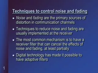
Techniques to control noise and fading. Noise and fading are the primary sources of distortion in communication channels Techniques to reduce noise and fading are usually implemented at the receiver

E N D
Techniques to control noise and fading • Noise and fading are the primary sources of distortion in communication channels • Techniques to reduce noise and fading are usually implemented at the receiver • The most common mechanism is to have a receiver filter that can cancel the effects of noise and fading, at least partially • Digital technology has made it possible to have adaptive filters
Principle of Equalization • Equalization is the process of compensation at the receiver, to reduce noise effects • The channel is treated as a filter with transfer function • Equalization is the process of creating a filter with an inverse transfer function of the channel • Since the channel is a varying filter, equalizer filter also has to change accordingly, hence the term adaptive.
Equalization Model-Signal detection Carrier Transmitter Channel Receiver Front End IF Stage Message signal x(t) Detector Detected signal y(t)
Equalization model-Correction Reconstructed Signal nb(t) Decision Maker Equalizer + Equivalent Noise
Equalizer System EquationsDetected signaly(t) = x(t) * f(t) + nb(t)=> Y(f) = X(f) F(f) + Nb(f)Output of the Equalizer ^ d(t) = y(t) * heq(t)
Equalizer System EquationsDesired output ^ D(f) = Y(f) Heq(f) = X(f) => Heq(f) X(f) F(f) = X(f)=> Heq(f) F(f) = 1Heq(f) = 1/ F(f) => Inverse filter
System Equations Error MSE Error = Aim of equalizer: To minimize MSE error
Equalizer Operating Modes • Training • Tracking
Training and Tracking functions • The Training sequence is a known pseudo-random signal or a fixed bit pattern sent by the transmitter. The user data is sent immediately after the training sequence • The equalizer uses training sequence to adjust its frequency response Heq (f) and is optimally ready for data sequence • Adjustment goes on dynamically, it is adaptable equalizer
Block Diagram of Digital Equalizer Z-1 Z-1 Z-1 w2k w0k w1k wNk ∑ - + ∑ Adaptive Algorithm
Digital Equalizer equations • In discrete form, we sample signals at interval of ‘T’ seconds : t = k T; • The output of Equalizer is:
Error minimization • The adaptive algorithm is controlled by the error signal, The equalizer weights are varied until convergence is reached.
Types of equalizers • Linear Equalizers. • Non Linear Equalizers.
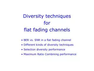
Diversity techniques • Powerful communications receiver technique that provides wireless link improvement at relatively low cost. • Unlike equalization, diversity requires no training overhead.
Principle of diversity • Small Scale fading causes deep and rapid amplitude fluctuations as mobile moves over a very small distances.
…Principle of diversity • If we space 2 antennas at 0.5 m, one may receive a null while the other receives a strong signal. By selecting the best signal at all times, a receiver can mitigate or reduce small-scale fading. This concept is Antenna Diversity.
Diversity Improvement • Consider a fading channel (Rayleigh) Input s(t) Output r(t) • Input-output relation r (t) = (t) e -j q(t) s (t) + n (t) • Average value of signal to noise ratio ___ SNR = = (Eb / No) 2 (t) Channel
Average SNR Improvement Using Diversity • p.d.f., p(γi) = (1 / ) e – γi / where (γi 0 ) and γi = instantaneous SNR Probability [γiγ] • M diversity branches, Probability [γi>γ]
Average Snr Improvement Using Diversity • Average SNR improvement using selection Diversity,
Example : Assume that 5 antennas are used to provide space diversity. If average SNR is 20 dB, determine the probability that the SNR will be 10 dB. Compare this with the case of a single receiver. Solution : = 20 dB => 100. Threshold γ = 10 dB = 10.
…Example Prob[γi>γ] = 1 – (1 – e – γ/ )M For M = 5, Prob= 1 – (1 – e – 0.1)5 = 0.9999 For M = 1(No Diversity), Prob= 1 – (1 – e – 0.1)= 0.905
Maximal Ratio Combining (MRC) • MRC uses each of the M branches in co-phased and weighted manner such that highest achievable SNR is available. If each branch has gain Gi, rM = total signal envelope =
…Maximal Ratio Combining (MRC) … assuming each branch has some average noise power N, total noise power NT applied to the detector is,
…Example e-0.1
Types of diversity • Space Diversity • Either at the mobile or base station. • At base station, separation on order of several tens of wavelength are required. • Polarization Diversity • Orthogonal Polarization to exploit diversity
…Types of diversity • Frequency Diversity : • More than one carrier frequency is used • Time Diversity : • Information is sent at time spacings • Greater than the coherence time of Channel, so multiple repetitions can be resolved
Practical diversity receiver – rake receiver • CDMA system uses RAKE Receiver to improve the signal to noise ratio at the receiver. • Generally CDMA systems don’t require equalization due to multi-path resolution.
Block Diagram Of Rake Receiver α1 M1 M2 M3α2 r(t) αM Z’ Z Correlator 1 ()dt Correlator 2 Σ Correlator M > < m’(t)
Principle Of Operation • M Correlators – Correlator 1 is synchronized to strongest multi-path M1. The correlator 2 is synchronized to next strongest multipath M2 and so on. • The weights 1 , 2 ,……,M are based on SNR from each correlator output. ( is proportional to SNR of correlator.) • M Z’ = M ZM m =1
…Principle Of Operation • Demodulation and bit decisions are then based on the weighted Outputs of M Correlators.