Network Analysis in Real World Systems: Bridging Centralities
Understand centralities in real-world networks, explore power law degree distribution, small world phenomenon, and robustness. Study different centrality measures like degree, closeness, betweenness, and Markov centrality. Examine network robustness and hierarchy. Investigate centralities like Bargain, PageRank, and Subgraph. Future works discussed.

Network Analysis in Real World Systems: Bridging Centralities
E N D
Presentation Transcript
Graph Element Analysis Woochang Hwang Department of Computer Science and Engineering State University of New York at Buffalo
Introduction • Real World Networks • Centralities • Motivation • Bridging Centrality • Bridge Cut • Discussion • Future Works
Introduction • Many real world systems can be described as networks. • Social relationships: e.g. collaboration relationships in academic, entertainment, business area. • Technological systems: e.g. internet topology, WWW, or mobile networks. • Biological systems: e.g. regulatory, metabolic, or interaction relationships. • Almost all of these real world networks are Scale-free.
Real World Networks Yeast PPI network
Real World Networks Proteom Size (PDB)
Real World Networks • Power law degree distribution: Rich get richer • Small World: A small average path length • Mean shortest node-to-node path • Can reach any nodes in a small number of hops, 5~6 hops • Robustness: Resilient and have strong resistance to failure on random attacks and vulnerable to targeted attacks • Hierarchical Modularity: A large clustering coefficient • How many of a node’s neighbors are connected to each other • Disassortative or Assortative • Biological networks: disassortative • Social networks: assortative
Real World Networks E. Ravasz et al.,Science, 2002
Protein Networks Real World Networks Metabolic Networks
node failure Real World Networks Complex systems maintain their basic functions even under errors and failures (cell mutations; Internet router breakdowns)
Robust. For <3, removing nodes does not break network into islands. Very resistant to random attacks, but attacks targeting key nodes are more dangerous. Real World Networks Max Cluster Size Path Length
Centralities • Degree centrality: number of direct neighbors of node v where N(v) is the set of direct neighbors of node v. • Stress centrality : the simple accumulation of a number of shortest paths between all node pairs where ρst(v) is the number of shortest paths passing through node v.
Centralities • Closeness centrality: reciprocal of the total distance from a node v to all the other nodes in a network δ(u,v) is the distance between node u and v. • Eccentricity: the greatest distance between v and any other vertex
Centralities • Shortest path based betweenness centrality : ratio of the number of shortest paths passing through a node v out of all shortest paths between all node pairs in a network σst is the number of shortest paths between node s and t and σst(v) is the number of shortest paths passing on a node v out σst • Current flow based betweenness centrality: the amount of current that flows through v in a network • Random walk based betweenness centrality
Centralities • Markov centrality: values for nodes show which node is closer to the center of mass. More central nodes can be reached from all other nodes in a shorter average time. where the mean first passage time (MFPT) msv in the Markov chain and n is |R|, R is a given root set. where n denotes the number of steps taken and denotes the probability that the chain starting at state s and first returns to state t in exactly n steps.
Centralities • Information centrality: incorporates the set of all possible paths between two nodes weighted by an information-based value for each path. where with Laplacian L and J=11T, and is the element on the sth row and sth column in CI. • It measures the harmonic mean length of paths ending at a vertex s, which is smaller if s has many short paths connecting it to other vertices. • Random walk based closeness centrality is equivalent to information centrality
Centralities • Eigenvector centrality: a measure of importance of nodes in a network using the adjacency and eigenvector matrices. where CIV is a eigenvector and λ is an eigenvalue. Only the largest eigenvalue will generate the desired centrality measurement. • Hubbel Index, Katz status index, etc….
Centralities • Bargain Centraity: In bargaining situations, it is advantageous to be connected to those who have few options; power comes from being connected to those who are powerless. Being connected to powerful people who have many competitive trading partners weakens one’s own bargaining power. where α is a scaling factor, β is the influence parameter, A is the adjacency matrix, and is the n-dimentional vector in which every entry is 1.
Centralities • PageRank: link analysis that scores relatively importance of web pages in a web network. • The PageRank of a Web page is defined recursively; a page has a high importance if it has a large number of incoming links from highly important Web pages. • PageRank also can be viewed as a probability distribution of the likelihood that a random surfer will arrive at any particular page at certain time. • Hypertext Induced Topic Selection (HITS), etc….
Centralities • Subgraph centrality: accounts for the participation of a node in all sub graphs of the network. the number of closed walks of length k starting and ending node v in the network is given by the local spectral moments μk(v).
Observation • Scale-free networks, basic properties • Power law degree distribution • Small World • Robustness • Hierarchical Modularity • Disassortative or Assortative • There should be some bridging nodes/edges between modules in scale-free networks based on these observations, and we did recognize the bridging nodes/edges by visual inspection of small example networks. • Finding the bridging nodes/edges, which are locating between modules, is an interesting and important problem for many applications on many different fields. (Networks’ robustness, paths protection, effective targets finding, etc.)
Motivation • Existing measurements are not enough for identifying the bridging nodes/edges: those existing indices are dominated by degree of the node of interest. • Betweenness of an edge also have a strong inclination to attach onto high degree nodes. • High tendency of cluttering in the center of the network. So, it is hard to differentiate the bridging nodes/edges from other kinds of nodes/edges. • Our focus in this research is to target vulnerable and central components in a network from a totally different point of view.
Bridge • Bridge • A bridge should be located on an important path, e.g. shortest path. • A bridge should be located between modules. • The neighbor regions of a bridging node should have low range of public domain among them.
Betweenness and Bridging Coefficient • Betweenness: global importance of a node/edge from shortest paths viewpoint. • Bridging Coefficient: a measurement that measuring the extent how well a node or edge is located between well connected regions. • the average probability of leaving the direct neighbor sub-graph of a node v.
Bridging Coefficient Figure 1. Bridging Coefficient
Bridging Centrality Bridging Centrality is defined as the product of the rank of the betweenness and the rank of the bridging coefficient.
Application on a synthetic network Figure 2.Figure 2A and 2B shows the results of bridging and betweenness centrality in the synthetic network respectively. The network contained 162 nodes and 362 edges and was created by adding bridging nodes to three independently generated sub-networks. Figure 2C shows the results for a synthetic network wherein 500 nodes were added to each sub-graph in Figure 2A and containing the same bridging nodes.
Application on Web Network Examples Figure 3.Results for Web Networks: Figure 1A and 1B shows the results for the AT&T Web Network and RPI Web Network, respectively. The nodes with the highest 0-5th percentile of values for the bridging centrality are highlighted in red circles; the nodes with the lowest values of bridging centrality are the 85th-100th percentiles and are highlighted in white circles. The color map for the percentile values is shown in the Figure.
Application on Social Network Examples Figure 4. Results for Social Networks: Figure 2A and 2B shows the results for the Les Miserable Character Network and Physics Collaboration Network, respectively. The nodes with the highest 0-5th percentile of values for the bridging centrality are highlighted in red circles; the nodes with the lowest values of bridging centrality are the 85th-100th percentiles and are highlighted in white circles. The nodes corresponding to Valjean (V), Javert (J), Pontmercy (P) and Cosette (C) are labeled in Figure 4A. The nodes corresponding to Rothman (R), Redner (R2), Dodds (D), Krapivsky (K) and Stanley (S) are labeled in Figure 2B. The color map for the percentile values is shown in the Figure.
Application on Biological Network Examples • Figure 5.Results for Biological Networks: Figure 3A and 3B shows the results the Cardiac Arrest Network and Yeast Metabolic Network, respectively. The nodes corresponding to Src, Shc and Jak2 (J2) are labeled in Figure 3A. The nodes with the highest 0-5th percentile of values for the bridging centrality are highlighted in red circles; the nodes with the lowest values of bridging centrality are the 85th-100th percentiles and are highlighted in white circles. The color map for the percentile values is shown in the Figure.
Assessing Network Disruption, Structural Integrity and Modularity Figure 6. Sequential node removal analysis on the yeast metabolic network
Assessing Ability To Occupy Topological Position • Figure 7A shows the clique affiliation of the nodes detected by three metrics, the bridging centrality (black squares), degree centrality (open circles), betweenness centrality (black circles). Maximal cliques were identified in the Yeast PPI network, and then we measured whether the detected nodes for each metric are in the identified cliques or not. In Figure 7B, random betweenness between detected cliques was measured in the clique graph for each metric, bridging centrality (black squares), degree centrality (open circles), betweenness centrality (black circles). Figure 7C compares the number of singletons that were generated according to sequential node deletion for each metric such as bridging centrality (dot line), degree centrality (gray line), betweenness centrality (black line). The nodes with the highest values for each of these network metrics were sequentially deleted and enumerated the number of singletons that were produced.
Assessing Ability To Occupy Modulating Position Figure 8. The biological and the topological characteristics of the direct neighbors of the node ordered by two metrics, the bridging centrality (black bar),betweenness centrality (white bar). Figure 6(a) showsthe gene expression correlation on the direct neighborsof each percentile. Figure 6(b) shows the average clustering coeffcient of the nodes in each percentile.
Druggability • The nodes corresponding to SHC, SRC, and JAK2 had the highest, 2nd and 3rd highest bridging centrality values. • The target of receptor antagonist drugs such as losartan, also signals via SRC and SHC in cardiac fibroblasts (cardiac structural tissue). • JAK2 activation is a key mediator of aldosterone-induced angiotensin-converting enzyme expression; the latter is the target of drugs such as captopril, enapril and other angiotensin-converting enzyme inhibitors (related high blood pressure)
Druggability • C21 Steroid Hormone Metabolism Network • The metabolites with the highest values of bridging centrality were: i) Corticosterone, ii) Cortisol, iii) 11 β -Hydroxyprogesterone, iv) Pregnenolone and, v) 21-deoxy-cortisol. • Corticosterone and cortisol are produced by the adrenal glands and mediate the flight or fight stress response, which includes changes to blood sugar, blood pressure and immune modulation.
Druggability • Steroid Biosynthesis Network • The metabolites with the highest values of bridging centrality were: i) Presqualene diphosphate, ii) Squalene, iii) (S)-2,3-epoxy-squalene, iv) Prephytoene diphosphate and, v) Phytoene. • Anti-fungal agents, a promising target for anti-cholesterol drugs (25) and the anti-cholesterolemic activity
Bridge Cut Algorithm • Iterative Graph Partitioning Algorithm • Compute Bridging Centrality for each edge • Cut the highest bridging edge • Identify an isolated module as a cluster if the density of the isolated module is greater than a threshold.
Clustering Validation • F-measure • Davies-Bouldin Index where diam(Ci) is the diameter of cluster Ciand d(Ci ;Cj) is the distance between cluster Ciand Cj. So, d(Ci ;Cj)is small if cluster i and j are compact and theirs centers are far away from each other. Therefore, DB will have a small values for a good clustering.
Bridge Cut Table 1: Comparative analysis. Performance ofbridge cut method on DIP PPI dataset (2339 nodes, 5595 edges) is comparedwith seven graph clustering approaches (Maximal clique,quasi clique, Rives, minimum cut, Markov clustering,Samanta). The fourth column represents the average F-measure of the clusters for MIPS complex modules. The fifth column indicates the Davies-Bouldin cluster quality index. Comparisons are performed on the clusters with4 or more components.
Bridge Cut Table 2. Comparative analysis. Performance of bridgecut method on the school friendship dataset (551 nodes, 2066 edges) is comparedwith seven graph clustering approaches (Maximal clique,quasi clique, Rives, minimum cut, Markov clustering,Samanta). Column descriptions are the same as Table 1
Discussion • The recognition of the bridges should be very valuable information for many different applications on many different areas. • Identifying functional, physical modules, or key components using the bridging centrality will provide an effective and totally new way of looking at biological systems. • Discovering sub-communities or important components in social network system. • Network robustness improvement, network protection, and paths protection using bridging information. • Drug Target Identification
Future Works • Directed network • Complexity