Download
1 / 25
250 likes | 375 Vues
I’d like to provide a brief introduction to, and overview of, exploratory factor analysis : Introduce a dataset on homelessness , provided by John Summerlin of CUNY. Contrast Principal Components Analysis ( PCA ) and Exploratory Factor Analysis ( EFA ) of these same data.

E N D
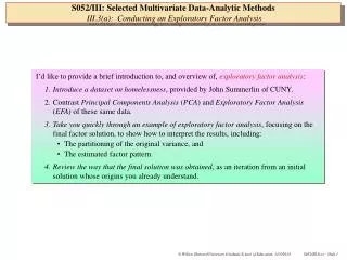
I’d like to provide a brief introduction to, and overview of, exploratory factor analysis: • Introduce a dataset on homelessness, provided by John Summerlin of CUNY. • Contrast Principal Components Analysis (PCA) and Exploratory Factor Analysis (EFA) of these same data. • Take you quickly through an example of exploratory factor analysis, focusing on the final factor solution, to show how to interpret the results, including: • The partitioning of the original variance, and • The estimated factor pattern. • Review the way that the final solution was obtained, as an iteration from an initial solution whose origins you already understand. S052/III: Selected Multivariate Data-Analytic MethodsIII.3(a): Conducting an Exploratory Factor Analysis
S052/III: Selected Multivariate Data-Analytic MethodsIII.3(a): Conducting an Exploratory Factor Analysis
Four observed indicators measuring the participant’s history of homelessness Two observed indicators of adaptive strength Indicators of depression and loneliness S052/III: Selected Multivariate Data-Analytic MethodsIII.3(a): Conducting an Exploratory Factor Analysis
Obtain univariate and bivariate descriptive information on the observed measures Handout III_3a_1 … First part of the PC-SAS program provides descriptive information… *----------------------------------------------------------------------------------* Input the dataset, name and label the variables *----------------------------------------------------------------------------------*; DATA HOMELESS; INFILE 'C:\DATA\S052\HOMELESS.txt'; INPUT ID AGE RACE ED LONGHOME TIMESHOM DURTHIS TIMEFST PAS SA DEPRESS ALONE; LABEL ID = 'Subject ID Number' AGE = 'Age' RACE = 'Race/Ethnicity' ED = 'Highest grade completed' LONGHOME = 'Longest time having a home since first homeless' TIMESHOM = 'Number of homeless episodes' DURTHIS = 'Duration of this homeless episode' TIMEFST = 'Time since first homeless episode' PAS = 'Personal Attitude' SA = 'Self-Actualization' DEPRESS = 'Depression' ALONE = 'Loneliness'; *----------------------------------------------------------------------------------* Obtain descriptive univariate and bivariate statistics on selected variables *----------------------------------------------------------------------------------*; PROC MEANS MIN MAX MEAN STD DATA=HOMELESS; VAR AGE ED LONGHOME TIMESHOM DURTHIS TIMEFST PAS SA DEPRESS ALONE; PROC CORR NOSIMPLE NOPROB DATA=HOMELESS; VAR LONGHOME TIMESHOM DURTHIS TIMEFST PAS SA DEPRESS ALONE; S052/III: Selected Multivariate Data-Analytic MethodsIII.3(a): Conducting an Exploratory Factor Analysis
Indicators display considerable variation in metric and variability. Age- and education-heterogeneous sample of men Variable Label Minimum Maximum ƒƒƒƒƒƒƒƒƒƒƒƒƒƒƒƒƒƒƒƒƒƒƒƒƒƒƒƒƒƒƒƒƒƒƒƒƒƒƒƒƒƒƒƒƒƒƒƒƒƒƒƒƒƒƒƒƒƒƒƒƒƒƒƒƒƒƒƒƒƒƒƒƒƒƒƒƒƒƒƒƒƒƒƒƒƒƒƒ AGE Age 19.0000000 60.0000000 ED Highest grade completed 4.0000000 19.0000000 LONGHOME Longest time having a home since first homeless 0 17.0000000 TIMESHOM Number of homeless episodes 1.0000000 98.0000000 DURTHIS Duration of this homeless episode 0.0192308 10.0000000 TIMEFST Time since first homeless episode 0.0192308 40.0000000 PAS Personal Attitude 213.0000000 347.0000000 SA Self-Actualization 41.0000000 81.0000000 DEPRESS Depression 5.0000000 20.0000000 ALONE Loneliness 5.0000000 20.0000000 ƒƒƒƒƒƒƒƒƒƒƒƒƒƒƒƒƒƒƒƒƒƒƒƒƒƒƒƒƒƒƒƒƒƒƒƒƒƒƒƒƒƒƒƒƒƒƒƒƒƒƒƒƒƒƒƒƒƒƒƒƒƒƒƒƒƒƒƒƒƒƒƒƒƒƒƒƒƒƒƒƒƒƒƒƒƒƒƒ Variable Label Mean Std Dev ƒƒƒƒƒƒƒƒƒƒƒƒƒƒƒƒƒƒƒƒƒƒƒƒƒƒƒƒƒƒƒƒƒƒƒƒƒƒƒƒƒƒƒƒƒƒƒƒƒƒƒƒƒƒƒƒƒƒƒƒƒƒƒƒƒƒƒƒƒƒƒƒƒƒƒƒƒƒƒƒƒƒƒƒƒƒƒƒ AGE Age 38.2479339 7.2895827 ED Highest grade completed 11.6198347 2.6370950 LONGHOME Longest time having a home since first homeless 1.5051282 2.5286911 TIMESHOM Number of homeless episodes 6.2436975 12.4580424 DURTHIS Duration of this homeless episode 1.2065705 1.7911078 TIMEFST Time since first homeless episode 8.0737444 8.1741362 PAS Personal Attitude 272.7916667 24.0118654 SA Self-Actualization 61.9421488 7.8105671 DEPRESS Depression 13.9833333 3.8084014 ALONE Loneliness 12.3833333 4.3679184 ƒƒƒƒƒƒƒƒƒƒƒƒƒƒƒƒƒƒƒƒƒƒƒƒƒƒƒƒƒƒƒƒƒƒƒƒƒƒƒƒƒƒƒƒƒƒƒƒƒƒƒƒƒƒƒƒƒƒƒƒƒƒƒƒƒƒƒƒƒƒƒƒƒƒƒƒƒƒƒƒƒƒƒƒƒƒƒƒ S052/III: Selected Multivariate Data-Analytic MethodsIII.3(a): Conducting an Exploratory Factor Analysis
Not all correlations are uniformly large There are clusters of more highly inter-correlated measures. • Not all correlations are uniformly positive • Need to be cautious because higher scores on some measures do not unilaterally imply “better”: • For instance, contrast SA and DEPRESS. • SA & ALONE, etc. Here are the bivariate correlations, estimated under pairwise deletion… Variable LONG TIME DUR TIME PAS SA DEP ALONE HOME SHOW THIS FST RESS ƒƒƒƒƒƒƒƒƒƒƒƒƒƒƒƒƒƒƒƒƒƒƒƒƒƒƒƒƒƒƒƒƒƒƒƒƒƒƒƒƒƒƒƒƒƒƒƒƒƒƒƒƒƒƒƒƒƒƒƒƒƒƒƒƒƒƒƒƒƒƒƒƒƒƒƒƒƒƒƒƒƒƒƒƒƒƒƒ LONGHOME 1.000 TIMESHOM 0.205 1.000 DURTHIS 0.269 0.228 1.000 TIMEFST 0.476 0.348 0.229 1.000 PAS -.047 -.085 -.091 -.185 1.000 SA 0.017 0.074 0.121 -.085 0.614 1.000 DEPRESS -.061 0.046 -.005 0.160 -.284 -.368 1.000 ALONE 0.057 0.021 -.079 0.105 -.313 -.447 0.517 1.000 ƒƒƒƒƒƒƒƒƒƒƒƒƒƒƒƒƒƒƒƒƒƒƒƒƒƒƒƒƒƒƒƒƒƒƒƒƒƒƒƒƒƒƒƒƒƒƒƒƒƒƒƒƒƒƒƒƒƒƒƒƒƒƒƒƒƒƒƒƒƒƒƒƒƒƒƒƒƒƒƒƒƒƒƒƒƒƒƒ S052/III: Selected Multivariate Data-Analytic MethodsIII.3(a): Conducting an Exploratory Factor Analysis
Rather than asking… Is there some sensible way to forge these several measures together into a smaller number of composites with defined properties? You can ask… Are there a number of unseen (latent) factors (constructs) acting “beneath” these measures to determine their observed values? Requires the use of …. Principal Components Analysis (PCA) Could use of …. Exploratory Factor Analysis (EFA) Question??? S052/III: Selected Multivariate Data-Analytic MethodsIII.3(a): Conducting an Exploratory Factor Analysis
A path model of principal components analysis… S052/III: Selected Multivariate Data-Analytic MethodsIII.3(a): Conducting an Exploratory Factor Analysis
A path model of factor analysis… S052/III: Selected Multivariate Data-Analytic MethodsIII.3(a): Conducting an Exploratory Factor Analysis
Model for Principal Components Analysis Model for Exploratory Factor Analysis Given the X’s, pick the a’s, and compute the PC’s Given the X’s, guess the ’s, guess the ’s, and compute the b’s A single set of answers An infinite number of equally correct answers Statistical Model S052/III: Selected Multivariate Data-Analytic MethodsIII.3(a): Conducting an Exploratory Factor Analysis
Principal Components Analysis Model Exploratory Factor Analysis Model Given the X’s, guess the ’s, guess the ’s, and compute the b’s Given the X’s, pick the a’s, and compute the PC’s A single set of answers An infinite number of equally correct answers Given the data, the answer is determined by the method and there are thousands of different methods of exploratory factor analysis… The answer is determined by the data Statistical Model S052/III: Selected Multivariate Data-Analytic MethodsIII.3(a): Conducting an Exploratory Factor Analysis
Re-orders the estimated factor loadings in the output, in order of magnitude (see later) • Ways of obtaining the initial factor solution (of either the covariance or the correlation matrix) in PC-SAS: • Alpha factor analysis, • Harris component analysis, • Image component analysis, • ML factor analysis, • Principal axis factoring, • Specified by user, • Unweighted least-squares factor analysis. • Ways of rotating to a final factor solution in PC-SAS: • Equamax, • Harris-Kaiser Ortho-oblique, • Orthomax, • Parsimax, • Procrustes, • Promax, • Quartimax, • Varimax. • Ways of obtaining initial estimates of the measurement error variance in PC-SAS: • Absolute SMC method, • Input from external file, • Maximum absolute correlation, • Set to one, • Set to random, • SMC. ( ) 2 7 6 8 Then, in Handout III_3a_1, comes the exploratory factory analysisPC-SAS programming… <input data steps and descriptive analyses omitted> *----------------------------------------------------------------------------------* Conduct a Principal Axis Factor analysis of selected variables, w/ Varimax Rotation *----------------------------------------------------------------------------------*; PROC FACTOR DATA=HOMELESS ROTATE=VARIMAX REORDER; VAR LONGHOME TIMESHOM DURTHIS TIMEFST PAS SA DEPRESS ALONE; S052/III: Selected Multivariate Data-Analytic MethodsIII.3(a): Conducting an Exploratory Factor Analysis
Although you cannot tell from this page, PROC FACTOR has standardized each of the original measures before proceeding with the EFA It has estimated and removed measurement error variance from each measure’s observed variability It has adopted a two-factor solution It has “rotated” to a final factor solution Glancing at the “final factor solution,” notice that PC_SAS has made several important decisions… Rotated Factor Pattern Factor1 Factor2 SA Self-Actualization 0.82469 0.08675 PAS Personal Attitude 0.71155 -0.13824 DEPRESS Depression -0.71400 0.00082 ALONE Loneliness -0.75301 -0.00786 TIMEFST Time since first homeless episode -0.16651 0.77044 LONGHOME Longest time having a home since first homeless -0.01135 0.73086 TIMESHOM Number of homeless episodes -0.03346 0.64533 DURTHIS Duration of this homeless episode 0.13315 0.58936 Variance Explained by Each Factor Factor1 Factor2 2.3100 1.9182 Final Communality Estimates Total = 4.2282 LONGHOME TIMESHOM DURTHIS TIMEFST PAS SA DEPRESS ALONE 0.5343 0.4176 0.3651 0.6213 0.5254 0.6876 0.5098 0.5671 S052/III: Selected Multivariate Data-Analytic MethodsIII.3(a): Conducting an Exploratory Factor Analysis
The estimation of coefficients related to the loadings linking the hypothesized factors to the original measures. The partitioning of the variability available from the standardized original measures There are actually two main parts to the final factor solution, that we will examine separately… Rotated Factor Pattern Factor1 Factor2 SA Self-Actualization 0.82469 0.08675 PAS Personal Attitude 0.71155 -0.13824 DEPRESS Depression -0.71400 0.00082 ALONE Loneliness -0.75301 -0.00786 TIMEFST Time since first homeless episode -0.16651 0.77044 LONGHOME Longest time having a home since first homeless -0.01135 0.73086 TIMESHOM Number of homeless episodes -0.03346 0.64533 DURTHIS Duration of this homeless episode 0.13315 0.58936 Variance Explained by Each Factor Factor1 Factor2 2.3100 1.9182 Final Communality Estimates Total = 4.2282 LONGHOME TIMESHOM DURTHIS TIMEFST PAS SA DEPRESS ALONE 0.5343 0.4176 0.3651 0.6213 0.5254 0.6876 0.5098 0.5671 S052/III: Selected Multivariate Data-Analytic MethodsIII.3(a): Conducting an Exploratory Factor Analysis
The original 8 units of standardized variance in the observed measures 4.2282 units of “communal” (shared) variance that is a consequence of the factor structure “common” to all observed measures The (8 - 4.2282) = 3.7718 units of variance that is “unexplained” by the factor structure remains “specific” or “unique” to the original measures = + “Communal Variance” “Specific Variance” “Original Variance” This 4.2282 units of communal (shared) variance is due to the presence of the underlying factors: 2.3100 units due to 1 + 1.9182 units due to 2 -------- 4.2282communal units Here’s an interpretation of the estimated partitioning of variance… Variance Explained by Each Factor Factor1 Factor2 2.3100 1.9182 Final Communality Estimates Total = 4.2282 LONGHOME TIMESHOM DURTHIS TIMEFST PAS SA DEPRESS ALONE 0.5343 0.4176 0.3651 0.6213 0.5254 0.6876 0.5098 0.5671 S052/III: Selected Multivariate Data-Analytic MethodsIII.3(a): Conducting an Exploratory Factor Analysis
8 units of original standardized variance 4.2282 units of communal (shared) variance (8 - 4.2282) = 3.7718 units of specific (unique) variance = + By subtraction, the portion of the original variances remaining specific (unique) to each of the original measures is: (1 - 0.5343) = 0.4657 units in X1 (1 - 0.4175) = 0.5825 units in X2 (1 - 0.3651) = 0.6349 units in X3 (1 - 0.6213) = 0.3787 units in X4 (1 - 0.5254) = 0.4746 units in X5 (1 - 0.6876) = 0.3124 units in X6 (1 - 0.5098) = 0.4902 units in X7 + (1 - 0.5671) = 0.4329 units in X8 -------- 3.7718specific units A portion of the standardized variance from each of the original measures contributes to the total communal variance of 4.2282 units 0.5343 units from to X1 0.4175 units from to X2 0.3651 units from to X3 0.6213 units from to X4 0.5254 units from to X5 0.6876 units from to X6 0.5098 units from to X7 + 0.5671 units from to X8 -------- 4.2282communal units Variance Explained by Each Factor Factor1 Factor2 2.3100 1.9182 Final Communality Estimates Total = 4.2282 LONGHOME TIMESHOM DURTHIS TIMEFST PAS SA DEPRESS ALONE 0.5343 0.4176 0.3651 0.6213 0.5254 0.6876 0.5098 0.5671 S052/III: Selected Multivariate Data-Analytic MethodsIII.3(a): Conducting an Exploratory Factor Analysis
Then, these are the estimated ‘true” variances, and also the estimated reliabilities, of the original measures If these are the estimated error variances of each of the original measures Variance Explained by Each Factor Factor1 Factor2 2.3100 1.9182 Final Communality Estimates Total = 4.2282 LONGHOME TIMESHOM DURTHIS TIMEFST PAS SA DEPRESS ALONE 0.5343 0.4176 0.3651 0.6213 0.5254 0.6876 0.5098 0.5671 S052/III: Selected Multivariate Data-Analytic MethodsIII.3(a): Conducting an Exploratory Factor Analysis 8 units of original standardized variance 4.2282 units of communal (shared) variance (8 - 4.2282) = 3.7718 units of specific (unique) variance = + By subtraction, the portion of the original variances remaining specific (unique) to each of the original measures is: (1 - 0.5343) = 0.4657 units in X1 (1 - 0.4175) = 0.5825 units in X2 (1 - 0.3651) = 0.6349 units in X3 (1 - 0.6213) = 0.3787 units in X4 (1 - 0.5254) = 0.4746 units in X5 (1 - 0.6876) = 0.3124 units in X6 (1 - 0.5098) = 0.4902 units in X7 + (1 - 0.5671) = 0.4329 units in X8 -------- 3.7718specific units A portion of the standardized variance from each of the original measures contributes to the total communal variance of 4.2282 units 0.5343 units from to X1 0.4175 units from to X2 0.3651 units from to X3 0.6213 units from to X4 0.5254 units from to X5 0.6876 units from to X6 0.5098 units from to X7 + 0.5671 units from to X8 -------- 4.2282communal units
These are not exactly the “factor loadings” – the b’s – referred to in the earlier factor model, but are derived directly from them. • To help in interpretation, EFA “standardizes” the loadings, using its knowledge of communal and specific variance, so that the rotated factor pattern can be interpreted as a set of correlations between the original measures and the factors: • Estimated correlation of SA and Factor1 is 0.8246, • Estimated correlation of SA and Factor2 is 0.0868, • Estimated correlation of PAS and Factor1 is 0.7116, • etc. • Inspection of the rotated factor pattern helps you interpret the factors that were detected: • Any correlation that is larger than .3, .4, .5, .. is “big”????? And here’s an interpretation of the estimated measure/factor relationship… Rotated Factor Pattern Factor1 Factor2 SA Self-Actualization 0.82469 0.08675 PAS Personal Attitude 0.71155 -0.13824 DEPRESS Depression -0.71400 0.00082 ALONE Loneliness -0.75301 -0.00786 TIMEFST Time since first homeless episode -0.16651 0.77044 LONGHOME Longest time having a home since first homeless -0.01135 0.73086 TIMESHOM Number of homeless episodes -0.03346 0.64533 DURTHIS Duration of this homeless episode 0.13315 0.58936 S052/III: Selected Multivariate Data-Analytic MethodsIII.3(a): Conducting an Exploratory Factor Analysis
People who score high on Factor2: • Have been homeless a long time, • Have had a home for a longer period since first homeless (??!!), • Have been homeless a lot, • Have had a longer current episode of homelessness • People who score high on Factor1: • Strive for more self-actualization, • Are more self-actualized, • Are less depressed, • Are less lonely. Summerlin (pp. 309-311) regards Factor1 as a construct that represents Adaptive Striving. Summerlin (pp. 309-311) regards Factor2 as a construct that represents Detachment. And here’s an interpretation of the estimated measure/factor relationship… Rotated Factor Pattern Factor1 Factor2 SA Self-Actualization 0.82469 0.08675 PAS Personal Attitude 0.71155 -0.13824 DEPRESS Depression -0.71400 0.00082 ALONE Loneliness -0.75301 -0.00786 TIMEFST Time since first homeless episode -0.16651 0.77044 LONGHOME Longest time having a home since first homeless -0.01135 0.73086 TIMESHOM Number of homeless episodes -0.03346 0.64533 DURTHIS Duration of this homeless episode 0.13315 0.58936 S052/III: Selected Multivariate Data-Analytic MethodsIII.3(a): Conducting an Exploratory Factor Analysis
These are not the “fundamental vectors of homelessness” (to paraphrase Spearman). • They are simply a parsimonious (and otherwise unconfirmed) way of “explaining” the origins of the 47% of the standardized variance shared in common by a specific collection of observed measures. • It’s the original choice of the measures, and the selected factor analytic method, that determines the underlying factor structure detected. Notice that there is nothing “absolute” or “universally true” about the factor solution. S052/III: Selected Multivariate Data-Analytic MethodsIII.3(a): Conducting an Exploratory Factor Analysis
They were obtained by Principal Axis Factoring (PAF): • PAF was the first kind of exploratory factor analysis developed, by Spearman. • PAF was developed soon after PCA had been invented.. • PAF estimates are obtained by turning PCA on its head! Examine the “Initial Factor Method” that we have so far ignored, on p. 4 of Handout III_3a_1 How were these estimates, communal and specific variances, and rotated factor patterns obtained? S052/III: Selected Multivariate Data-Analytic MethodsIII.3(a): Conducting an Exploratory Factor Analysis
Second, PAF treats all eight units of original standardized variance (ONE unit/measure) as eligible for factoring in the initial round of analysis. First, PAF uses Principal Components Analysis as a pre-cursor to the factor analysis! Third, PAF uses the Rule of One to determine the dimensionality of the data (2-D), and then treats the sum of the PC1 & PC2 eigenvalues (2.3345 + 1.8936 = 4.2281) as the communal “true” variance that will be explained by the hypothesized latent factor structure. Fourth, PAF treats the sum of the PC3 through PC8 eigenvalues (=3.7719) as the specific or unique “measurement error” variance that will not be explained by the hypothesized latent factor structure. Here is the initial part of the principal axis factoring that we have so far ignored …. S052/III: Selected Multivariate Data-Analytic MethodsIII.3(a): Conducting an Exploratory Factor Analysis Initial Factor Method: Principal Components Prior Communality Estimates: ONE Eigenvalues of the Correlation Matrix: Total = 8 Average = 1 Eigenvalue Difference Proportion Cumulative 1 2.33454113 0.44089636 0.2918 0.2918 2 1.89364477 0.98216332 0.2367 0.5285 3 0.91148145 0.05675118 0.1139 0.6425 4 0.85473028 0.07614386 0.1068 0.7493 5 0.77858642 0.25899985 0.0973 0.8466 6 0.51958657 0.14092901 0.0649 0.9116 7 0.37865756 0.04988573 0.0473 0.9589 8 0.32877183 0.0411 1.0000 2 factors will be retained by the MINEIGEN criterion.
EFA then takes the initial “two component” PCA solution: Inverts it to make the X’s the subject of the formulae: Initial set of correlations of X1 thru X8 with Factor1 and Factor2 The values of the b’s are computed algebraically from the values of the a’s, which are known from the original PCA. Initial Factor Method: Principal Components Factor Pattern Factor1 Factor2 ALONE Loneliness 0.72986 -0.18547 DEPRESS Depression 0.69400 -0.16782 PAS Personal Attitude -0.72407 0.03371 SA Self-Actualization -0.78088 0.27905 TIMEFST Time since first homeless episode 0.34374 0.70933 LONGHOME Longest time having a home since first homeless 0.18362 0.70751 TIMESHOM Number of homeless episodes 0.18491 0.61918 DURTHIS Duration of this homeless episode 0.00979 0.60414 S052/III: Selected Multivariate Data-Analytic MethodsIII.3(a): Conducting an Exploratory Factor Analysis
_ _ X1 X2 • Then, seek another pair of rotated axes that provide “better” values for the loadings: • Varimax rotation seeks a new axes on which the loadings are close to a maximum or close to zero. X5 X7 X6 X8 _ _ _ _ X3 X4 Obtain “rotated” loadings by projection onto the new axes, and print out as the “rotated factor pattern” matrix. _ _ Then, the initial solution is “rotated” to an “optimum” final solution …. First, plot the loadings from the initial factor pattern in the space defined by initialFactor1 and Factor2. Factor1 S052/III: Selected Multivariate Data-Analytic MethodsIII.3(a): Conducting an Exploratory Factor Analysis Factor2
There are a remarkable number of ad-hoc decisions made when an exploratory factor analysis is conducted! For this reason alone, it is perhaps not worth trusting…? However, confirmatory factor analysis is different – rather than rambling around looking for any kind of solution, it proposes a particular hypothesized factor structure for the data and tests to see if the hypothesis can be rejected. • S-090: • Answering Complex Questions • with Multivariate Methods One thing should be very clear from all of this…. S052/III: Selected Multivariate Data-Analytic MethodsIII.3(a): Conducting an Exploratory Factor Analysis