Machine Learning: Connectionist

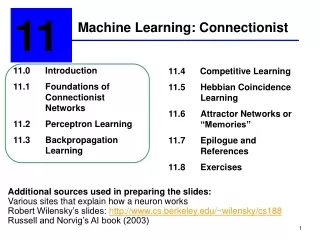
1. 11 Machine Learning: Connectionist 11.0 Introduction 11.1 Foundations of Connectionist Networks 11.2 Perceptron Learning 11.3 Backpropagation Learning 11.4 Competitive Learning 11.5 Hebbian Coincidence Learning 11.6 Attractor Networks or “Memories” 11.7 Epilogue and References 11.8 Exercises Additional sources used in preparing the slides: Various sites that explain how a neuron works Robert Wilensky’s slides: http://www.cs.berkeley.edu/~wilensky/cs188Russell and Norvig’s AI book (2003)

2. Chapter Objectives • Learn about • the neurons in the human brain • single neuron systems (perceptrons) • neural networks

3. Inspiration: The human brain • We seem to learn facts and get better at doing things without having to run a separate “learning procedure.” • It is desirable to integrate learning more with doing.

4. Understanding the brain (1) • “ Because we do not understand the brain very well we are constantly tempted to use the latest technology as a model for trying to understand it. In my childhood we were always assured that the brain was a telephone switchboard. (“What else could it be?”) I was amused to see that Sherrington, the great British neuroscientist, thought that the brain worked like a telegraph system. Freud often compared the brain to hydraulic and electro-magnetic systems. Leibniz compared it to a mill, and I am told that some of the ancient Greeks thought the brain functions like a catapult. At present, obviously, the metaphor is the digital computer.” -- John R. Searle (Prof. of Philosophy at UC, Berkeley)

5. Understanding the brain (2) • “ The brain is a tissue. It is a complicated, intricately woven tissue, like nothing else we know of in the universe, but it is composed of cells, as any tissue is. They are, to be sure, highly specialized cells, but they function according to the laws that govern any other cells. Their electrical and chemical signals can be detected, recorded and interpreted and their chemicals can be identified, the connections that constitute the brain’s woven feltwork can be mapped. In short, the brain can be studied, just as the kidney can. -- David H. Hubel (1981 Nobel Prize Winner)

6. The brain • The brain doesn’t seem to have a CPU. • Instead, it’s got lots of simple, parallel, asynchronous units, called neurons. • There are about 1011 neurons of about 20 types

7. Neurons • Every neuron is a single cell that has a number of relatively short fibers, called dendrites, and one long fiber, called an axon. • The end of the axon branches out into more short fibers • Each fiber “connects” to the dendrites and cell bodies of other neurons • The “connection” is actually a short gap, called a synapse • Axons are transmitters, dendrites are receivers • There are about 1014 connections

8. Neuron

9. How do neurons work • The fibers of surrounding neurons emit chemicals (neurotransmitters) that move across the synapse and change the electrical potential of the cell body • Sometimes the action across the synapse increases the potential, and sometimes it decreases it. • If the potential reaches a certain threshold, an electrical pulse, or action potential, will travel down the axon, eventually reaching all the branches, causing them to release their neurotransmitters. And so on ...

10. How do neurons work (cont’d)

11. How do neurons change • There are changes to neurons that are presumed to reflect or enable learning: • The synaptic connections exhibit plasticity. In other words, the degree to which a neuron will react to a stimulus across a particular synapse is subject to long-term change over time (long-term potentiation). • Neurons also will create new connections to other neurons. • Other changes in structure also seem to occur, some less well understood than others.

12. Neurons as devices • Neurons are slow devices. • Tens of milliseconds to do something. (1ms – 10ms cycles time) • Feldman translates this into the “100 step program constraint”: Most of the AI tasks we want to do take people less than a second. So any brain “program” can’t be longer than 100 neural “instructions.” • No particular unit seems to be important. Destroying any one brain cell has little effect on overall processing.

13. How do neurons do it? • Basically, all the billions of neurons in the brain are active at once. So, this is truly massive parallelism. • But, probably not the kind of parallelism that we are used to in conventional Computer Science. • Sending messages (i.e., patterns that encode information) is probably too slow to work. • So information is probably encoded some other way, e.g., by the connections themselves.

14. AI / Cognitive Science Implication • Explain cognition by richly connected networks transmitting simple signals. • Sometimes called • Connectionist computing (by Jerry Feldman) • Parallel Distributed Processing (PDP)(by Rumelhart, McClelland, and Hinton) • Neural networks (NN) • Artificial neural networks (ANN)(emphasizing that the relation to biology is generally rather tenuous)

15. From a neuron to a perceptron • All connectionist models use a similar model of a neuron • There is a collection of units each of which has • a number of weighted inputs from other units • inputs represent the degree to which the other unit is firing • weights represent how much the units wants to listen to other units • a threshold that the sum of the weighted inputs are compared against • the threshold has to be crossed for the unit to do something (“fire”) • a single output to another bunch of units • what the unit decided to do, given all the inputs and its threshold

16. Notes • The perceptrons are continuously active - Actually, real neurons fire all the time; what changes is the rate of firing, from a few to a few hundred impulses a second • The weights of the perceptrons are not fixed - Indeed, learning in a NN system is basically a matter of changing the weights

17. A unit (perceptron) w0 x0 • xi are the inputs wi are the weightsw0 is usually set for the threshold with x0 =-1 (bias)in is the weighted sum of inputs including the threshold (activation level)g is the activation functiona is the activation or the output. The output is computed using a function that determines how far the perceptron’s activation level is below or above 0 w1 x1 w2 x2 a= g(in) . . . in=wixi wn xn

18. A single perceptron’s computation • A perceptron computes a = g (X . W), • where • in = X.W = w0 * -1 + w1 * x1 + w2 * x2 + … + wn * xn, • and g is (usually) the threshold function: g(z) = 1 if z > 0 and 0 otherwise • A perceptron can act as a logic gate interpreting 1 as true and 0 (or -1) as false • Notice in the definition of g that we are using z>0 rather than z≥0.

19. Logical function and 1.5 -1 x+y-1.5 x  y 1 x 1 y

20. Logical function or 0.5 -1 x+y-0.5 x V y 1 x 1 y

21. Logical function not -0.5 -1 0.5 - x ¬x -1 x

22. Interesting questions for perceptrons • How do we wire up a network of perceptrons? - i.e., what “architecture” do we use? • How does the network represent knowledge? - i.e., what do the nodes mean? • How do we set the weights? - i.e., how does learning take place?

23. Training single perceptrons • We can train perceptrons to compute the function of our choice • The procedure • Start with a perceptron with any values for the weights (usually 0) • Feed the input, let the perceptron compute the answer • If the answer is right, do nothing • If the answer is wrong, then modify the weights by adding or subtracting the input vector (perhaps scaled down) • Iterate over all the input vectors, repeating as necessary, until the perceptron learns what we want

24. Training single perceptrons: the intuition • If the unit should have gone on, but didn’t, increase the influence of the inputs that are on: - adding the inputs (or a fraction thereof) to the weights will do so. • If it should have been off, but was on, decrease influence of the units that are on: - subtracting the input from the weights does this. • Multiplying the input vector by a number before adding or subtracting scales down the effect. This number is called the learning constant.

25. Example: teaching the logical or function • Want to learn this: • Initially the weights are all 0, i.e., the weight vector is (0 0 0). • The next step is to cycle through the inputs and change the weights as necessary.

26. Walking through the learning process • Start with the weight vector (0 0 0) • ITERATION 1 • Doing example (-1 0 0 0) The sum is 0, the output is 0, the desired output is 0. The results are equal, do nothing. • Doing example (-1 0 1 1) The sum is 0, the output is 0, the desired output is 1. Add half of the inputs to the weights. The new weight vector is (-0.5 0 0.5).

27. Walking through the learning process • The weight vector is (-0.5 0 0.5) • Doing example (-1 1 0 1) The sum is 0.5, the output is 1, the desired output is 1. The results are equal, do nothing. • Doing example (-1 1 1 1) The sum is 1, the output is 1, the desired output is 1. The results are equal, do nothing.

28. Walking through the learning process • The weight vector is (-0.5 0 0.5) • ITERATION 2 • Doing example (-1 0 0 0) The sum is 0.5, the output is 1, the desired output is 0. Subtract half of the inputs from the weights. The new weight vector is (0 0 0.5). • Doing example (-1 0 1 1) The sum is 0.5, the output is 1, the desired output is 1. The results are equal do nothing.

29. Walking through the learning process • The weight vector is (0 0 0.5) • Doing example (-1 1 0 1) The sum is 0, the output is 0, the desired output is 1. Add half of the inputs to the weights. The new weight vector is (-0.5 0.5 0.5) • Doing example (-1 1 1 1) The sum is 1.5, the output is 1, the desired output is 1. The results are equal, do nothing.

30. Walking through the learning process • The weight vector is (-0.5 0.5 0.5) • ITERATION 3 • Doing example (-1 0 0 0) The sum is 0.5, the output is 1, the desired output is 0. Subtract half of the inputs from the weights. The new weight vector is (0 0.5 0.5). • Doing example (-1 0 1 1) The sum is 0.5, the output is 1, the desired output is 1. The results are equal do nothing.

31. Walking through the learning process • The weight vector is (0 0.5 0.5) • Doing example (-1 1 0 1) The sum is 0.5, the output is 1, the desired output is 1. The results are equal, do nothing. • Doing example (-1 1 1 1) The sum is 1.5, the output is 1, the desired output is 1. The results are equal, do nothing.

32. Walking through the learning process • The weight vector is (0 0.5 0.5) • ITERATION 4 • Doing example (-1 0 0 0) The sum is 0, the output is 0, the desired output is 0. The results are equal do nothing. • Doing example (-1 0 1 1) The sum is 0.5, the output is 1, the desired output is 1. The results are equal do nothing.

33. Walking through the learning process • The weight vector is (0 0.5 0.5) • Doing example (-1 1 0 1) The sum is 0.5, the output is 1, the desired output is 1. The results are equal, do nothing. • Doing example (-1 1 1 1) The sum is 1.5, the output is 1, the desired output is 1. The results are equal, do nothing. • Converged after 3 iterations! • Notice that the result is different from the original design for the logical or.

34. A data set for perceptron classification

35. A two-dimensional plot of the data points

36. The results of perceptron training • The weight vector converges to (-6.0 -1.3 -0.25)after 5 iterations. • The equation of the line found is -1.3 * x1 + -0.25 * x2 + -6.0 = 0 • The Y intercept is 24.0, the X intercept is 4.6.(considering the absolute values)

37. The bad news: the exclusive-or problem • No straight line in two-dimensions can separate the (0, 1) and (1, 0) data points from (0, 0) and (1, 1). • A single perceptron can only learn linearly separable data sets (in any number of dimensions).

38. The solution: multi-layered NNs

39. Comments on neural networks • Parallelism in AI is not new. - spreading activation, etc. • Neural models for AI is not new. - Indeed, is as old as AI, some subdisciplines such as computer vision, have continuously thought this way. • Much neural network works makes biologically implausible assumptions about how neurons work • backpropagation is biologically implausible • “neurally inspired computing” rather than “brain science.”

40. Comments on neural networks (cont’d) • None of the neural network models distinguish humans from dogs from dolphins from flatworms. Whatever distinguishes “higher” cognitive capacities (language, reasoning) may not be apparent at this level of analysis. • Relation between neural networks and “symbolic AI”? • Some claim NN models don’t have symbols and representations. • Others think of NNs as simply being an “implementation-level” theory. NNs started out as a branch of statistical pattern classification, and is headed back that way.

41. Nevertheless • NNs give us important insights into how to think about cognition • NNs have been used in solving lots of problems • learning how to pronounce words from spelling (NETtalk, Sejnowski and Rosenberg, 1987) • Controlling kilns (Ciftci, 2001)