Connectionist Modeling
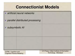
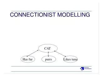
Connectionist Modeling. Some material taken from cspeech.ucd.ie/~connectionism and Rich & Knight, 1991. What is Connectionist Architecture? . Very simple neuron-like processing elements. Weighted connections between these elements. Highly parallel & distributed.

Connectionist Modeling
E N D
Presentation Transcript
Connectionist Modeling Some material taken from cspeech.ucd.ie/~connectionism and Rich & Knight, 1991
What is Connectionist Architecture? • Very simple neuron-like processing elements. • Weighted connections between these elements. • Highly parallel & distributed. • Emphasis on learning internal representations automatically.
What is Good About Connectionist Models? • Inspired by the brain. • Neuron-like elements & synapse-like connections. • Local, parallel computation. • Distributed representation. • Plausible experience-based learning. • Good generalization via similarity. • Graceful degradation.
Inspired by the Brain • The brain is made up of areas. • Complex patterns of projections within and between areas. • Feedforward (sensory -> central) • Feedback (recurrence)
Neurons • Input from many other neurons. • Inputs sum until a threshold reached. • At threshold, a spike is generated. • The neuron then rests. • Typical firing rate is 100 Hz (computer is 1,000,000,000 Hz)
Synapses • Axons almost touch dendrites of other neurons. • Neurotransmitters effect transmission from cell to cell through synapse. • This is where long term learning takes place.
Synapse Learning • One way the brain learns is by modification of synapses as a result of experience. • Hebb’s postulate (1949): • When an axon of cell A … excites cell B and repeatedly or persistently takes part in firing it, some growth process or metabolic change takes place in one or both cells so that A’s efficiency as one of the cells firing B is increased. • Bliss and Lomo (1973) discovered this type of learning in the hippocampus.
Local, Parallel Computation • The net input is the weighted sum of all incoming activations. • The activation of this unit is some function of net, f.
Local, Parallel Computation 1 .2 -.4 -1 .9 -.4 -.4 -.4 .3 1 -.4 net = 1*.2 + -1*.9 + 1*.3 = -.4 f(x) = x
Simple Feedforward Network units weights
Mapping from input to output input layer 0.5 1.0 -0.1 0.2 Input pattern: <0.5, 1.0,-0.1,0.2>
Mapping from input to output hidden layer 0.2 -0.5 0.8 input layer 0.5 1.0 -0.1 0.2 Input pattern: <0.5, 1.0,-0.1,0.2>
feed-forward processing Mapping from input to output Output pattern: <-0.9, 0.2,-0.1,0.7> output layer -0.9 0.2 -0.1 0.7 hidden layer 0.2 -0.5 0.8 input layer 0.5 1.0 -0.1 0.2 Input pattern: <0.5, 1.0,-0.1,0.2>
Early Network Models • McClelland and Rummelhart’s model of Word Superiority effect • Weights hand crafted.
Perceptrons • Rosenblatt, 1962 • 2-Layer network. • Threshold activation function at output • +1 if weighted input is above threshold. • -1 if below threshold.
Perceptrons x1 w1 x2 w2 . . . wn xn
Perceptrons x0=1 w0 x1 w1 . . . wn xn
Perceptrons x0=1 1 if g(x) > 0 0 if g(x) < 0 w0 x1 w1 g(x)=w0+x1w1+x2w2 w2 x2
Perceptrons • Perceptrons can learn to compute functions. • In particular, perceptrons can solve linearly separable problems. B A and B B A B xor B A
x0=1 w0 x1 w1 . . . wn xn Perceptrons • Perceptrons are trained on input/output pairs. • If fires when shouldn’t, make each wi smaller by an amount proportional to xi. • If doesn’t fire when should, make each wi larger.
Perceptrons 1 -.06 0 -.1 0 .05 -.06 0 RIGHT
Perceptrons 1 -.06 0 -.1 1 .05 -.01 0 RIGHT
Perceptrons 1 -.06 1 -.1 0 .05 -.16 0 RIGHT
Perceptrons 1 -.06 1 -.1 1 .05 -.11 0 WRONG
Perceptrons Fails to fire, so add proportion, , to weights. 1 -.06 -.1 .05
Perceptrons 1 = .01 -.06+.01x1 -.1+.01x1 .05+.01x1
Perceptrons 1 -.05 -.09 .06 nnd4pr
Gradient Descent • Choose some (random) initial values for the model parameters. • Calculate the gradient G of the error function with respect to each model parameter. • Change the model parameters so that we move a short distance in the direction of the greatest rate of decrease of the error, i.e., in the direction of -G. • Repeat steps 2 and 3 until G gets close to zero.
Adding Hidden Units 1 input space 0 1 hidden unit space
Minsky & Papert • Minsky & Papert (1969) claimed that multi-layered networks with non-linear hidden units could not be trained. • Backpropagation solved this problem.
For each pattern in the training set: Compute the error at the output nodes Compute Dw for each wt in 2nd layer Compute delta (generalized error expression) for hidden units Compute Dw for each wt in 1st layer Backpropagation After amassing Dw for all weights and all patterns, change each wt a little bit, as determined by the learning rate nnd12sd1 nnd12mo
Benefits of Connectionism • Link to biological systems • Neural basis. • Parallel. • Distributed. • Good generalization. • Graceful degredation. • Learning. • Very powerful and general.
Problems with Connectionism • Intrepretablility. • Weights. • Distributed nature. • Faithfulness. • Often not well understood why they do what they do. • Often complex. • Falsifiability. • Gradient descent as search. • Gradient descent as model of learning.