Download
1 / 47
480 likes | 624 Vues
Simple learning in connectionist networks. Learning associations in connectionist networks Associationism (James, 1890) Association by contiguity Generalization by similarity. Connectionist implementation

E N D
Learning associations in connectionist networks Associationism (James, 1890) Association by contiguity Generalization by similarity Connectionist implementation Represent items as patterns of activity, where similarity is measured in terms of overlap/correlation of patterns Represent contiguity of items as simultaneous presence of their patterns over two groups of units (A and B) Adjust weights on connections between units in A and units in B so that the pattern on A tends to cause the corresponding pattern on B As a result, when we next present the same or similar pattern on A, it tends to produce the corresponding pattern on B (perhaps somewhat weakened or distorted)
Correlational learning: Hebb rule What Hebb actually said: When an axon of cell A is near enough to excite a cell B and repeatedly and consistently takes part in firing it, some growth process or metabolic change takes place in one or both cells such that A’s efficacy, as one of the cells firing B, is increased. The minimal version of the Hebb rule: When there is a synapse between cell A and cell B, increment the strength of the synapse whenever A and B fire together (or in close succession). The minimal Hebb rule as implemented in a network:
So weight from sending to receiving unit ends up being proportional to their correlation over patterns…
Lawrence Jennifer Aniston Face perception units Postle Brad Pitt
Face perception neurons (“Sending units”) “Synapses” Name neurons (“receiving units”)
Simple learning model • Imagine neurons have a threshold set at 0. If input is above threshold (positive number), the neuron fires strongly. If it is below threshold (negative number), the neuron fires weakly. • When a face is directly observed, the features it possesses get positive input, all others get negative input. • When a name is presented, it gets positive input, all others get negative input.
Face perception neurons Brad Pitt Name neurons
Face perception neurons Brad Postle Name neurons
Learning to name faces • Goal: Encode “memory” of which name goes with which name… • …so, when given face, correct name units activate. • Face units are “sending units”, name units are “receiving units” • Synapse has a “weight” that describes effect of sending unit on receiving unit • Negative weight= inhibitory influence, positive weight = excitatory influence • Activation rule for name units: • Take state of sending unit * value of synapse (weight), summed over all sending units to get net input. • Activate strongly if net input >0, otherwise activate weakly.
Face perception neurons Name neurons
Face perception neurons Brad Pitt Name neurons
Face perception neurons Name neurons
Face perception neurons Brad Postle Name neurons
Face perception neurons Name neurons Brad Postle
Face perception neurons Name neurons Brad Pitt
Face perception neurons Name neurons Not Brad Pitt or Postle
Face perception neurons Jennifer Aniston Name neurons
Face perception neurons Jennifer Lawrence Name neurons
Face perception neurons Name neurons
With Hebbian learning, many different patterns can be stored in a single configuration of weights. • What would happen if we kept training this model with the same four faces? • Same weight configuration, just with larger weights.
Hebbian learning • Captures “contiguity” of learning (things that occur together should become associated in memory) • Learning rule (∆wij = ε aj ai) is proportional to correlation coefficient between units. • Captures effects of “similarity” in learning (a learned response should generalize to things with similar representations) • With linear units (ai = neti), output is a weighted sum of the unit’s previous activation to stored patterns… • …where the “weight” in the sum is proportional to the similarity (dot product) between the current input pattern and the previously stored pattern • So, a test pattern that is completely dissimilar to a stored pattern (dot product of zero) will not be affected by the stored pattern at all.
Limitations of Hebbian learning • Many association problems it cannot solve • Especially where similar input patterns must produce quite different outputs. • Without further constraints, weights grow without bound • Each weight is learned independently of all others • Weight changes are exactly the same from pass to pass.
Error-correcting learning (delta rule)
Face perception neurons Brad Pitt Squared error! Name neurons Error! Target states
3 w1 w2 1 2
Delta-rule learning with linear units • Captures intuition that learning should reduce discrepancy between what you predict and what actually happens (error). • Basic approach: Measure error for current input/output pair; compute derivative of this error with respect to each weight; change weight by small amount to reduce error. • For squared error, change in weight is proportional to (tj – aj) ai • …that is, the correlation between the input activation and the current error. • Weight changes can be viewed as performing “gradient descent” in error (each change will reduce total error). • Algorithm is inherently multi-pass: changes to a given weight will vary from pass to pass, b/c error depends on state of weights.
Delta rule will learn any association for which a solution exists!