Probability
E N D
Presentation Transcript
Probability • Statistical inference is based on a Mathematics branch called probability theory. • If a procedure can result in n equally likely outcomes, nA of which have attribute A, then we say that attribute A has probability nA/n, and we write P(A) = nA/n.
Probability • Consider a true die tossed fairly: • The probability of an even numbered outcome (2, 4, or 6) is ½. • nA =3 • N = 6 • P(A) = 3/6 = ½.
Probability • Concept of equally likely is the basis of the probability. • Experiment can be broken into sets of basic outcomes, no one of which is more likely to occur than any other.
Probability • Suppose a penny and a nickel are tossed together, what is the probability of getting two heads? Equally likely outcomes 1 2 3 4 Penny H T H T Nickel H H T T • P(2H) = ¼.
Probability Rules Principles of Enumeration • Multiplication Principle • If an event occur in a ways and if a second event occur in b ways independent of the way in which the first event occurred, then the two events together can occur in a.b ways.
Multiplication Principle • A clinical lab has 4 methods to determine serum cholesterol and 2 methods to determine blood glucose level, then the patient’s serum cholesterol and blood glucose can be determined in 4.2 ways. • Cholesterol level: I II III IV • Glucose level: 1 2 • Patient: I1 I2 II1 II2 III1 III2 IV1 IV2
2. An Addition Principle • If one event can occur in a ways and if a second event can occur in b ways, then one or the other of the events can occur in a + b ways, provided the two events can not occur together.
An Addition Principle • 2 cancer patients • 5 heart patients need to be bathe by the nurse • The nurse can choose any patient to bathe first; she has 2 + 5 = 7 ways to choose her first patients. • Exception is the patient should not have the two diseases together, Exclusivity.
Semantic Aid • In multiplication principle, events are: event 1 and event 2 • While in addition principle, they are: event 1 or event 2. • And implies multiplication • Or implies addition.
Probability of Composite Events Independent Events (Multiplication) • If a procedure can result in n equally likely outcomes, nA of which have attribute A, then we say that attribute A has probability nA/n, and we write P(A) = nA/n. • If a procedure can result in n equally likely outcomes, nA of which have attribute B, then we say that attribute B has probability nB/n, and we write P(B) = nB/n.
Independent Events • Composite event A and B: • P (A and B) = nA . nB /n2 = nA/n . nB/n = P(A) . (P(B) • To hold this, outcome of the event B must not depend upon the outcome of the vent A. • That is events A and B are independent.
Independent Events • Two events A and B are independent if P (A and B) = P(A) . (P(B) • A fair coin is tossed, find the prob. of two heads: • P(head on first) = ½, P(head on second) = ½ • And P(head on first) . P(head on second) = ½. ½ = ¼. • P (2 heads) = HH, HT, TH, TT = ¼.
Mutually Exclusive Events Addition • Probability of event Aor event B • If A can occur in nA ways and if B can occur in nB ways and if A and B can not occur together, then the number of equally likely outcomes favorable to A or B is: nA + nB • P(A or B) = nA + nB / n = nA/n + nB/n = P(A) + P(B).
Mutually Not Exclusive Events • nA + nB – n A and B • P(A or B) = nA + nB– n A and B n • = nA/n + nB/n – n A and B /n • P(A or B) = P(A) + P(B) – P (A and B)
Addition Example • Find the probability of drawing a jack or a heart from a well shuffled deck of 52 cards. • A: drawing a jack • B: drawing a heart • A and B: drawing a jack and a heart (i,e., drawing the jack of hearts)
Addition Example • P(A) = 4/52 = 1/13 • P(B) = 13/52 = 1/4 • P (A and B) = 1/52 • P(A or B) = P(A) + P(B) – P (A and B) • P(A or B) = 1/13 + ¼ - 1/52 = 16/52
Marginal, Joint and Conditional Probability Cross classification by age and sex of 100 residents Sex 70-79 80-89 90&over Total Male 20 10 10 40 Female 30 20 10 60 Total 50 30 20 100
Marginal Events • What is the probability of selecting a male? • P (selecting a male) = 40/100 = 0.4 • P (selecting an 80 to 90 year old) = 30/10 = 0.3
Marginal Probability • If n equally likely outcomes of a procedure are cross-classified according to two or more classification variables and if the specification of an event fails to mention one or more of the classification variables, then such an event is called a marginal event and its probability is called a marginal probability.
Joint Event • Probability of selecting a male who is also 80 to 90 years old. • The event jointly specify the sex and age and is referred as joint event and its probability is joint probability.
Joint Probability • P (male and 80-90) = 10/100 = 0.1 • P (female and 80-90) = 20/100 = 0.2
Joint Probability • If n equally likely outcomes of a procedure are cross-classified according to two or more classification variables and if the specification of an event requires simultaneous occurrence of the two classification variables, then such an event is called a joint event and its probability is called a joint probability.
Conditional Events • A substudy of female population • Within female population, the probability of selecting 80 to 90 years old? • = 20/60 = 0.33 • Reduced set of equally likely outcomes • P (80-89 female) = 1/3 • P (female 80-89) = 1/3 ? = 20/30 = 2/3
Conditional Probability • P (90&over male) = 10/40 = ¼ • P (male 90&over) = 10/20 = ½
Conditional Probability • Events of the form “A given B” state that the occurrence of A given that B must occur are called conditional events. Their probabilities are called conditional probabilities and are denoted by P(A B), provided that P(B) = 0. • The restriction B must be different from zero is important.
Conditional Probability • Consider the event 80-89 given female • P(80-90 female) = 1/3 = 20/100 /60/100 • = P(80-90 and female) /P (female) • Numerator joins age and sex, a joint event and can be generalized for any two events: P(A B) = P(A and B) /P(B) • When B is zero, it will be an undefined function.
Conditional Probability • P(A B) = P(A and B) /P(B) • P(A B) = P(A and B) /P(B) = P(A).P(B) P(B) • P(A B) = P(A), if the two events (A and B) are independent
Conditional Probability • P(B A) = P(B and A) /P(A), A = 0 • P(B A) = P(B and A) /P(A) = P(B).P(A) P(A) • P(B A) = P(B), if the two events (B and A) are independent
Summary • P(A B) = P(A and B) /P(B), if B is not zero • P(B A) = P(B and A) /P(A), if A is not zero • Two events “A and B” and “B and A” are identical thus having same probabilities, P(B and A) = P(A and B). • P(B A) = P(B and A) /P(A) = P(A and B) /P(A), multiplying both sides by P(A), • P(A and B) = P(A) . P(B A)
Summary • P(A or B) = P(A) + P(B) – P(A and B) • P(A or B) = P(A) + P(B), if A and B are mutually exclusive. • P(A and B) = P(A) . P(B A) • P(A and B) = P(A) . P(B), if A and B are independent.
Probability Requirements • Requirements for the probability distribution of a discrete random variable x: • P(x) 0 for all values of x • P(x) <0 for all values of x • p(x) = 1 • x, denotes the absence of x, that is the occurrence of “not x”, then P(x) + P(x) = 1 or P(x) = 1 – P(x), x and x are complimentary All x
Baye’s Rule • P(A B) and P(B A) are two different events and in general are not equal, such as if B is some effect and A is a cause, then P(B A) is the prob. of effect given cause, when we want to know the P(A B), prob. of cause given effect. • Physician may know the prob. of a particular symptoms given a particular disease, but wants to know the prob. of disease given the observed symptoms for a patient?
Baye’s Rule • Let D denote the disease and S the symptoms. • If D is the presence of the disease, D denote its absence. • P(D) + P(D) = 1, P(D) = 1 - P(D) • P(S D) and P(S D), symptoms with or without disease. • P(D S) = ?
Baye’s Rule • P(S) = P(S and D) + P(S and D), mutually exclusive • P(S D) = P(S and D) / P(D) and P(S D) = P(S and D) / P(D), multiply by P(D) and P(D), respectively. • P(S and D) = P(D).P(S D) and P(S and D) = P(D).P(S D)
Baye’s Rule • P(D S) = P(D and S) / P(S) = P(S and D) P(S and D) + P(S and D) or P(D S) = P(D) . P(S D) P(D) . P(S D) + P(D) . P(S D) quantities assumed to be known
Baye’s Rule • This expression is commonly known as Baye’s rule, named after Reverend Thomas Bayes (1702-1761).
Baye’s Rule • Cancer in women over 40 • Prevalence or P(D) = 1% = 0.01 • Test sensitivity 95% or 0.95 • Test specificity 3% or 0.03 • P(D = 0.01 • P(D) = 0.99 • P(S D) = 0.95 • P(S D) = 0.03
Baye’s Rule • P(D S) = (0.01) (0.95) (0.01) (0.95) + (0.99) (0.03) = 0.24, predictive value (low #)
Baye’s Rule • 100,000 women, prevalence rate 1% • 1000 women will have disease • Test sensitivity is 95%, 950 will screen positive, 50 negative (false negative) • 99,000 women disease free • Test specificity 97% = 0.97*99,000 = 96,030 screen negative • 99,000 – 96,030 = 2970 false positive
Baye’s Rule With disease Without Disease Total Screened positive 950 2970 3,920 Screened negative 50 96,030 96,080 Total 1,000 99,000 100,000 Yield (predictive value) = 950 / (950+2970) = 950/3920 = 0.24
Baye’s Rule With disease Without Disease Total Screened positive a b a+b Screened negative c d c+d Total a+c b+d N
Baye’s Rule • Prevalence Rate = a+c /N • Sensitivity = a /a+c • Specificity = d /b+d • False + rate = b /b+d • False – rate = c /a+c • Yield or predictive value = a /a+b
Baye’s Rule Yield = P(D S) = P(D) . P(S D) P(D) . P(S D) + P(D) . P(S D) = (prevalence) (sensitivity) (prevalence) (sensitivity) + (1-prevalence)(1-sensitivity)
Baye’s Rule • For t distinct disease states D1, D2,…,Dt, such that: ∑ P(Di) = 1 P(Dj S) = P(Dj) . P(S Dj) ∑ P(Di) . P(S Di) t i=1 t i=1
