Response Time
Response Time. Introduction. Example. Physician office. Patients arrive, on average, every five minutes - It takes ten minutes to serve a patient - Patients are willing to wait What is the implied utilization of the barber shop? How long will patients have to wait?. Example.

Response Time
E N D
Presentation Transcript
Response Time Introduction
Example Physician office • Patients arrive, on average, every five minutes- It takes ten minutes to serve a patient- Patients are willing to wait • What is the implied utilization of the barber shop? • How long will patients have to wait?
Example Physician office • Patients arrive, on average, every five minutes- It takes four minutes to serve a patient- Patients are willing to wait • What is the utilization of the barber shop? • How long will patients have to wait?
A Somewhat Odd Service Process Arrival Time Service Time Patient 1 0 4 2 5 4 3 10 4 4 15 4 5 20 4 6 25 4 7 30 4 8 35 4 9 40 4 10 45 4 11 50 4 12 55 4 7:00 7:10 7:20 7:30 7:40 7:50 8:00
A More Realistic Service Process Arrival Time Service Time Patient 1 0 5 2 7 6 3 9 7 4 12 6 5 18 5 6 22 2 7 25 4 8 30 3 9 36 4 10 45 2 11 51 2 12 55 3 Patient 1 Patient 3 Patient 5 Patient 7 Patient 9 Patient 11 Patient 2 Patient 4 Patient 6 Patient 8 Patient 10 Patient 12 Time 7:00 7:10 7:20 7:30 7:40 7:50 8:00 3 2 Number of cases 1 0 2 min. 3 min. 4 min. 5 min. 6 min. 7 min. Service times
Variability Leads to Waiting Time Arrival Time Service Time Patient 1 0 5 2 7 6 3 9 7 4 12 6 5 18 5 6 22 2 7 25 4 8 30 3 9 36 4 10 45 2 11 51 2 12 55 3 Service time Wait time 7:00 7:10 7:20 7:30 7:40 7:50 8:00 5 4 3 2 1 Inventory (Patients at lab) 0 7:00 7:10 7:20 7:30 7:40 7:50 8:00
The Curse of Variability - Summary Variability hurts flow With buffers: we see waiting times even though there exists excess capacity Variability is BAD and it does not average itself out New models are needed to understand these effects
Response Time Waiting time models: The need for excess capacity
Modeling Variability in Flow Flow Rate Minimum{Demand, Capacity} = Demand = 1/a Outflow No loss, waiting only This requires u<100% Outflow=Inflow Processing Buffer Inflow Demand process is “random” Look at the inter-arrival times a: average inter-arrival time CVa = Often Poisson distributed: CVa = 1 Constant hazard rate (no memory) Exponential inter-arrivals Difference between seasonality and variability • Processing • p: average processing time • Same as “activity time” and “service time” • CVp = • Can have many distributions: • CVp depends strongly on standardization • Often Beta or LogNormal IA1 IA2 IA3 IA4 Time St-Dev(processing times) St-Dev(inter-arrival times) Average(processing times) Average(inter-arrival times)
The Waiting Time Formula Increasing Variability Average flow time T Flow rate Inventory waiting Iq Inflow Outflow Entry to system Begin Service Departure Time in queue Tq Service Time p Theoretical Flow Time Flow Time T=Tq+p Utilization 100% Waiting Time Formula Variability factor Utilization factor Service time factor
Example: Walk-in Doc Newt Philly needs to get some medical advise. He knows that his Doc, Francoise, has a patient arrive every 30 minutes (with a standard deviation of 30 minutes). A typical consultation lasts 15 minutes (with a standard deviation of 15 minutes). The Doc has an open-access policy and does not offer appointments. If Newt walks into Francois’s practice at 10am, when can he expect to leave the practice again?
Summary Even though the utilization of a process might be less than 100%, it might still require long customer wait time Variability is the root cause for this effect As utilization approaches 100%, you will see a very steep increase in the wait time If you want fast service, you will have to hold excess capacity
Response Time More on Waiting time models / Staffing to Demand
Waiting Time Formula for Multiple, Parallel Resources Inventory in service Ip Inventory waiting Iq Outflow Inflow Flow rate Entry to system Begin Service Departure Time in queue Tq Service Time p Flow Time T=Tq+p Waiting Time Formula for Multiple (m) Servers
Example: Online retailer • Customers send emails to a help desk of an online retailer every 2 minutes, on average, and the standard deviation of the inter-arrival time is also 2 minutes. The online retailer has three employees answering emails. It takes on average 4 minutes to write a response email. The standard deviation of the service times is 2 minutes. • Estimate the average customer wait before being served.
Summary of Queuing Analysis Flow unit Server Utilization (Note: make sure <1) Inventory in service Ip Time related measures Inventory waiting Iq Outflow Inflow Inventory related measures (Flow rate=1/a) Entry to system Begin Service Departure Waiting Time Tq Service Time p Flow Time T=Tq+p
Staffing Decision • Customers send emails to a help desk of an online retailer every 2 minutes, on average, and the standard deviation of the inter-arrival time is also 2 minutes. The online retailer has three employees answering emails. It takes on average 4 minutes to write a response email. The standard deviation of the service times is 2 minutes. • How many employees would we have to add to get the average wait time reduced to x minutes?
What to Do With Seasonal Data Measure the true demand data Apply waiting model in each slice Slice the data by the hour (30min, 15min) Level the demand Assume demand is “stationary” within a slice
Service Levels in Waiting Systems Fraction of customers who have to wait xseconds or less 1 90% of calls had to wait 25 seconds or less Waiting times for those customers who do not get served immediately 0.8 0.6 Fraction of customers who get served without waiting at all 0.4 0.2 0 0 50 100 150 200 Waiting time [seconds] • Target Wait Time (TWT) • Service Level = Probability{Waiting TimeTWT} • Example: Big Call Center - starting point / diagnostic: 30% of calls answered within 20 seconds - target: 80% of calls answered within 20 seconds
Response Time Capacity Pooling
Managerial Responses to Variability: Pooling Independent Resources 2x(m=1) • Example: • Processing time=4 minutes • Inter-arrival time=5 minutes (at each server) • m=1, Cva=CVp=1 • Tq = • Processing time=4 minutes • Inter-arrival time=2.5 minutesm=2, Cva=CVp=1 • Tq = Pooled Resources (m=2)
Managerial Responses to Variability: Pooling Waiting Time Tq 70.00 m=1 60.00 50.00 40.00 m=2 30.00 20.00 m=5 10.00 m=10 0.00 60% 65% 70% 75% 80% 85% 90% 95% Utilization u
Summary What is a good wait time? Fire truck or IRS?
Limitations of Pooling Assumes flexibility Increases complexity of work-flow Can increase the variability of service time Interrupts the relationship with the customer / one-face-to-the-customer Group clinics Electricity grid / smart grid Flexible production plants
The Three Enemies of Operations Additional costs due to variability in demand and activity times Is associated with longer wait times and / or customer loss Requires process to hold excess capacity (idle time) Variability Inflexibility Customerdemand • Additional costs incurred because of supply demand mismatches • Waiting customers or • Waiting (idle capacity) Capacity • Use of resources beyond what is needed to meet customer requirements • Not adding value to the product, but adding cost • Reducing the performance of the production system • 7 different types of waste Waste Work Waste Value- adding Work Waste Value- adding
Response Time Scheduling / Access
Managerial Responses to Variability: Priority Rules in Waiting Time Systems • Flow units are sequenced in the waiting area (triage step) • Provides an opportunity for us to move some units forwards and some backwards • First-Come-First-Serve - easy to implement - perceived fairness - lowest variance of waiting time • Sequence based on importance - emergency cases - identifying profitable flow units
A A C C B B D D Managerial Responses to Variability: Priority Rules in Waiting Time Systems Service times: A: 9 minutesB: 10 minutesC: 4 minutesD: 8 minutes 4 min. 9 min. 19 min. 12 min. 23 min. 21 min. Total wait time: 9+19+23=51min Total wait time: 4+13+21=38 min • Shortest Processing Time Rule - Minimizes average waiting time - Problem of having “true” processing times
Appointments • Open Access • Appointment systems
Response Time Redesign the Service Process
Reasons for Long Response Times (And Potential Improvement Strategies) • Insufficient capacity on a permanent basis=> Understand what keeps the capacity low • Demand fluctuation and temporal capacity shortfalls • Unpredictable wait times => Extra capacity / Reduce variability in demand • Predictable wait times => Staff to demand / Takt time • Long wait times because of low priority=> Align priorities with customer value • Many steps in the process / poor internal process flow (often driven by handoffs and rework loops)=> Redesign the service process http://www.minyanville.com/businessmarkets/articles/drive-thrus-emissions-fast-food-mcdonalds/5/12/2010/id/28261
The Customer’s Perspective How much time does a patient spend on a primary care encounter? 20 minutes Driving Parking Check-in Vitals Waiting PCP Appt. Check out Labs Drive home Two types of wasted time: Auxiliary activities required to get to value add activities (result of process location / lay-out) Wait time (result of bottlenecks / insufficient capacity) Total value add time of a unit Total time a unit is in the process Flow Time Efficiency (or %VAT) =
Process Mapping / Service Blue Prints Customer supplies more data Walk into the branch / talk to agent Sign contracts Customer supplies more data Customer actions Line of interaction Collect basic information Request for more data Explain final document Onstage actions Request for more data Line of visibility Pre Approval process; set up workflow / account responsibility Pre Approval process; set up workflow / account responsibility Backstage actions Line of internal interaction Run formal credit scoring model Support processes Source: Yves Pigneur
Process Mapping / Service Blue PrintsHow to Redesign a Service Process Move work off the stage Example: online check-in at an airport Reduce customer actions / rely on support processes Example: checking in at a doctor’s office Instead of optimizing the capacity of a resource, try to eliminate the step altogether Example: Hertz Gold – Check-in offers no value; go directly to the car Avoid fragmentation of work due to specialization / narrow job responsibilities Example: Loan processing / hospital ward If customers are likely to leave the process because of long wait times, have the wait occur later in the process / re-sequence the activities Example: Starbucks – Pay early, then wait for the coffee Have the waiting occur outside of a line Example: Restaurants in a shopping malls using buzzers Example: Appointment Communicate the wait time with the customer (set expectations) Example: Disney
Response Time Loss Models
Different Models of Variability Waiting problems Utilization has to be less than 100% Impact of variability is on Flow Time Loss problems Demand can be bigger than capacity Impact of variability is on Flow Rate Pure waitingproblem, all customersare perfectly patient. All customers enter the process,some leave due totheir impatience Customers do notenter the process oncebuffer has reached a certain limit Customers are lostonce all servers arebusy Same if customers are patient Same if buffer size=0 Same if buffer size is extremely large Variability is always bad – you pay through lower flow rate and/or longer flow time Buffer or suffer: if you are willing to tolerate waiting, you don’t have to give up on flow rate
Analyzing Loss Systems Resources 3 trauma bays (m=3) Ambulances / Helicopters Trauma center moves to diversion status once all servers are busy incoming patients are directed to other locations Demand Process One trauma case comes in every 3 hours (a=3 hours) a is the interarrival time Exponential interarrival times Service Process Patient stays in trauma bayfor an average of 2 hours (p=2 hours) p is the service time Can have any distribution What is Pm, the probability that all m resources are utilized?
Analyzing Loss Systems: Finding Pm(r) • Given Pm(r) we can compute: • Time per day that system has to deny access • Flow units lost = 1/a * Pm (r) m • Define r = p / a • Example: r= 2 hours/ 3 hours r=0.67 • Recall m=3 • Use Erlang Loss Table • Find that P3 (0.67)=0.0255 r = p / a
Implied utilization vs probability of having all servers utilized: Pooling Revisited 0.6 Probabilitythat all serversare utilized 0.5 0.4 m=1 m=2 0.3 0.2 m=3 m=5 m=10 0.1 m=20 0 0 0.1 0.2 0.3 0.4 0.5 0.6 0.7 0.8 0.9 1 1.1 Implied utilization
Erlang Loss Table Probability{all m servers busy}=
Response Time Review
(My-law.com) My-law.com is a recent start-up trying to cater to customers in search of legal services online. Unlike traditional law firms, My-law.com allows for extensive interaction between lawyers and their customers via telephone and the Internet. This process is used in the upfront part of the customer interaction, largely consisting of answering some basic customer questions prior to entering a formal relationship. In order to allow customers to interact with the firm’s lawyers, customers are encouraged to send e-mails to my-lawyer@My-law.com. From there, the incoming e-mails are distributed to the lawyer who is currently “on call.” Given the broad skills of the lawyers, each lawyer can respond to each incoming request. E-mails arrive from 8 A.M. to 6 P.M. at a rate of 10 e-mails per hour (coefficient of variation for the arrivals is 1). At each moment in time, there is exactly one lawyer “on call,” that is, sitting at his or her desk waiting for incoming e-mails. It takes the lawyer, on average, 5 minutes to write the response e-mail. The standard deviation of this is 4 minutes. a. What is the average time a customer has to wait for the response to his/her e-mail, ignoring any transmission times? Note: This includes the time it takes the lawyer to start writing the e-mail and the actual writing time. b. How many e-mails will a lawyer have received at the end of a 10-hour day? c. When not responding to e-mails, the lawyer on call is encouraged to actively pursue cases that potentially could lead to large settlements. How much time on a 10-hour day can a My-law.com lawyer dedicate to this activity
Jim’s Computer Jim wants to find someone to fix his computer. PC Fixers (PF) is a local service that offers such computer repairs. A new customer walks into PF every 10 minutes (with a standard deviation of 10 minutes). PF has a staff of 5 computer technicians. Service times average around 40 minutes (with a standard deviation of 40 minutes). JC1. If Jim walks into PF, how long must he wait in line before he can see a technician? (Only include the waiting time, not any service time) JC2. How many customers will, on average, be waiting for their computer to be fixed?
Real Compute RealCompute offers real-time computing services. The company owns 4 supercomputers that can be accessed through the internet. Their customers send jobs that arrive on average every 4 minutes (inter-arrival times are exponentially distributed and, thus, the standard deviation of the inter-arrival times is 4 minutes). Each job takes on average 10 minutes of one of the supercomputers (during this time, the computer cannot perform any other work). Customers pay $20 for the execution of each job. Given the time-sensitive nature of the calculations, if no supercomputer is available, the job is redirected to a supercomputer of a partner company called OnComp, which charges $40 per job to Real Compute (OnComp always has supercomputer capacity available). RC1. What is the probability with which an incoming job can be executed by one of the supercomputers owned by RealCompute? RC2. How much does RealCompute pay on average to OnComp (in $s per hour)?
Contractor A contractor building houses and doing renovation work has currently six projects planned for the season. Below are the items, and the estimated times to complete them: New construction at Springfield - 60 days Bathroom remodeling at Herne - 10 days Training time for solar roof installation - 2 days Update web-site - 6 days Renovation of deck at Haverford - 8 days New kitchen at Rosemont - 20 days Suppose the contractor starts immediately with the first project, no other projects get added to this list, and the contractor sequences them so as to minimize the average time the project waits before it gets started. What will the contractor be doing in 30 days from the start date of the first project?
Call Center Consider a call center that has a constant staffing level. Because of increased demand in the morning, the call center has a very high utilization in the morning and a very low utilization in the afternoon. Which of the following will decrease the average waiting time in the call center? (a) Add more servers (b) Decrease the service time coefficient of variation (c) Decrease the average service time (d) Level the demand between the morning hours and the afternoon hours (e) All of the above