Multiple alignment: Feng-Doolittle algorithm
Multiple alignment: Feng-Doolittle algorithm. Why multiple alignments?. Alignment of more than two sequences Usually gives better information about conserved regions and function (more data) Better estimate of significance when using a sequence of unknown function

Multiple alignment: Feng-Doolittle algorithm
E N D
Presentation Transcript
Multiple alignment: Feng-Doolittle algorithm Bioinformatics I Fall 2002
Why multiple alignments? • Alignment of more than two sequences • Usually gives better information about conserved regions and function (more data) • Better estimate of significance when using a sequence of unknown function • Must use multiple alignments when establishing phylogenetic relationships Bioinformatics I Fall 2002
Dynamic programming extended to many dimensions? • No – uses up too much computer time and space • E.g. 200 amino acids in a pairwise alignment – must evaluate 4 x 10⁴ matrix elements • If 3 sequences, 8 x 10⁶ matrix elements • If 6 sequences, 6.4 x 10¹³ matrix elements Bioinformatics I Fall 2002
Need to find more efficient method • Sacrifice certainty of optimum alignment for certainty of good alignment but faster Bioinformatics I Fall 2002
Feng-doolittle algorithm • Does all pairwise alignments and scores them • Converts pairwise scores to “distances” • D = -logSeff = -log [(Sobs –Srand)/(Smax –Srand)] • Sobs = pairwise alignment score • Srand = expected score for random alignment • Smax = average of self-alignments of the two sequences Bioinformatics I Fall 2002
As Srand increases (increasing evolutionary distance), Seff goes down; this is why –log is used to scale Seff so that it’s linear with evolutionary distance. Bioinformatics I Fall 2002
Once the distances have been calculated, construct a guide tree (more in the phylogeny class) – tells what order to group the sequences • Sequences can be aligned with sequences or groups; groups can be aligned with groups Bioinformatics I Fall 2002
Sequence-sequence alignments: dynamic programming • Sequence-group alignments: all possible pairwise alignments between sequence and group are tried, highest scoring pair is how it gets aligned to group • Group-group alignments: all possible pairwise alignments of sequences between groups are tried; highest scoring pair is how groups get aligned Bioinformatics I Fall 2002
Example Seq5 Seq3 Seq4 Seq1 Seq2 Alignment 2 Alignment 1 Alignment 3 Final alignment Bioinformatics I Fall 2002
Notice that this method does not guarantee the optimum alignment; just a good one. Gaps are preserved from alignment to alignment: “once a gap, always a gap” Bioinformatics I Fall 2002
In-class exercise • Run Gap on all combinations of the sequences in multalign.rsf; penalize endgaps as before; use a gap penalty of 6 and an extension penalty of 2 • Record quality scores of each pairwise comparison Bioinformatics I Fall 2002
In class exercise, cont • use quality scores as distance measures; make a guide tree based on these scores • Select all sequences in multalign.rsf; select Functions multiple alignment pileup; select options, select penalize end gaps; set gap penalty at 6, gap extension at 2 • Compare pileup’s guide tree with yours Bioinformatics I Fall 2002
In class exercise, cont • Select pileup file in the output manager; select add to editor; select load second copy at the prompt • Carefully examine pileup’s alignment; compare it to the pairwise alignments (you can open them from the output manager) Bioinformatics I Fall 2002
Start refining alignment: • Use structural info if you have it • Find patterns if you don’t • Use amino acid structure handout from beginning of class for substitution decisions! Bioinformatics I Fall 2002
ClustalW • Most widely used multiple alignment method • Similar strategy to the Feng-Doolittle approach implemented as Pileup, but more complex and gives generally superior results • Ad hoc nature of the program can be mysterious Bioinformatics I Fall 2002
Advantageous differences • Gap penalties vary locally: • By observed frequency (in database) after each residue • By simple structure prediction – lower gap penalties in probable loop regions • By proximity to existing gaps – higher gap penalties when within 8 residues of an existing gap Bioinformatics I Fall 2002
Advantages, cont. • Change in substitution matrix choice depending on distance computed for guide tree • Substitution matrix families • Profile construction (more later) • Weighting of sequences in profiles depending on evolutionary distance computed for guide tree • More similar sequences get less weight than less similar sequences Bioinformatics I Fall 2002
In class exercise II • Change a few parameters in the ClustalW program (gap, gap extension, substitution matrix, etc.) one at a time: this is done in Alignment Setup. After each run with a different change, save the alignment project with some descriptive name that you can remember (e.g., gap20 or blosum) • Compare alignment results with different parameters changed Bioinformatics I Fall 2002
MultAlin • MultAlin is also a heuristic algorithm that builds up a multiple alignment from a group of pairwise alignments • It differs from Pileup and Clustal in that the guide tree is recalculated based on the results of each alignment step • Because this leads to cycles of tree building and alignmnent, MultAlin can take a long time to run. It stops after the overall alignment score stops improving Bioinformatics I Fall 2002
Scoring a multiple sequence alignment • Assumptions: • Sequences (rows) independent • Positions (columns) independent • Neither assumption is true … • Score of a column is the (possibly weighted) sum of all the pairwise comparisons (I.e., substitution matrix values) within that column • Score of a multiple alignment is the sum of scores for all columns Bioinformatics I Fall 2002
Introduction to profiles • A profile is a way to take into account variability in characters within each position in a msa • As you look along the column of a msa, you can see different characters • A profile is a way to preserve the information about the differences observed within each column Bioinformatics I Fall 2002
Profile building: simple model (Durbin, fig. 5.3) In column 1, we have 5 v’s, 1 f, and 1 i To score an “a” in that position in a sequence being tested for fit to the profile, we use the frequency information in the column vga--hagey v----nvdev vea--dvagh vkg------d vys--tyets fna--nipkh iagadngagv Bioinformatics I Fall 2002
Profile: simple model, cont. • Score for the alignment of that position is 5/7 s(v,a) + 1/7 s(f,a), + 1/7 s(i,a) where s(x,a) is the value from a substitution matrix for x substituted for a • Gap penalty decreased according to the length of the longest gap spanning that column • Idea is to maximize the score of the alignment of the new sequence to the profile (or reject an alignment that falls below a threshold) Bioinformatics I Fall 2002
Profile, evolutionary model • Instead of just estimating the probabilities found empirically to predict the probability of a different substitution, explicitly assume that everything seen in the column is a substitution from a common ancestor • This allows us to use Bayesian approaches about prior and posterior probabilities Bioinformatics I Fall 2002
Profile-type programs • Again, idea is to make a profile, then search for more sequences that fit that profile • Example: ProfileSearch, BLOCKS, etc. • Can combine this with statistical methods like expectation maximization (MEME) and Gibbs Sampler. Both of these depend on “random” starting points and algorithms that converge on an endpoint Bioinformatics I Fall 2002
In class exercise: Profilemake, etc. • Open nosalign.rsf file • Select 3 or 4 sequences; then use Edit select range, enter numbers for a range within these sequences (range of about 500 column positions) • Select Functions ProfileMake; choose use selected regions; take defaults and select run • Examine output Bioinformatics I Fall 2002
Now select ProfileSearch; use Query profiles pulldown to select the profilemake (.prf) output you just created; this profile will be the input for the Profile Search • The default database to search is SwissProt; we’ll leave it at the default, but you can use the Search set option to change or add to the databases searched (this is a local search) • Choose ProfileSegments; this will show local alignments between some number of the returned sequences with the profile • Choose run; this search will take a long time, perhaps 20 minutes Bioinformatics I Fall 2002
Other GCG profile programs • MEME: finds conserved motifs in a group of unaligned sequences • MotifSearch: uses output of MEME to search a database for new sequences Bioinformatics I Fall 2002
Confusingly named but related GCG programs • Motifs: searches a protein sequence for presence of motif patterns already identified in the Prosite library • ProfileScan: similar to Motifs, but uses profiles in the Prosite library to search the sequence for the presence of a profile; also performs the alignment of the profile to the sequence Bioinformatics I Fall 2002
Check out these websites for more • BLOCKS • eMOTIF • GIBBS • HMMER • SAGA Bioinformatics I Fall 2002
PAM matrices • Started with alignments of very closely related proteins; each pair of sequences was at least 85% identical • Then used idea of parsimony (least number of changes) to build phylogenetic trees acgctafki gcgctafki acgctafkl gcgctgfki gcgctlfki asgctafkl acactafkl Bioinformatics I Fall 2002
acgctafki il ag gcgctafki acgctafkl ag al cs ga gcgctgfki gcgctlfki acactafkl asgctafkl Bioinformatics I Fall 2002
For each amino acid, find the frequency Fi,j for which it is (reciprocally) substituted by every other amino acid • for example, Fg,a = 3 • Compute the relative mutability mi of each amino acid • the relative mutability is the number of times the amino acid is substituted by any other amino acid in the phylogenetic tree, divided by the number of mutations that could have affected the residue (times scaling factor 100) • for example, ma • number of times a substituted = 4 • number of mutations in entire tree x 2 = 12 • frequency of a = 10/63 = 0.159 • ma = 4/12 x 0.159 x 100 = 0.0209 Bioinformatics I Fall 2002
Compute the mutation probability Mij of each pair of amino acids • Mij = mjFij/SFij • SFij is the total number of substitutions involving a in the phylogenetic tree • Mg,a = 0.0209 x ¾ = 0.0156 (notice j refers to a) • Divide the mutation probability by the frequency of occurrence fi of residue i, and take the log • fi in this example is fg = 10/63 = 0.1587 • Rg,a = log (0.0156/0.1587) = 1.01 Bioinformatics I Fall 2002
Then defined a 1PAM (1 point accepted mutation) matrix to be one where the expected number of mutations overall was 1% (that’s why the factor of 100 is used). The entries in the whole matrix generated by the above method gives the PAM1 matrix; this supposes an amount of evolutionary time goes by that will let this amount of change happen Bioinformatics I Fall 2002
To get longer times, multiply PAM1 by itself by however many units of time you are interested in, e.g. PAM250 is PAM1 raised to the 250 power • So for PAM, higher numbers indicate longer evolutionary time Bioinformatics I Fall 2002
BLOSUM matrices • We’ll turn to the BLOSUM substitution matrices, because they were made using a special kind of profile called a block: areas of alignments that contain no gaps • We want to assign a score that gives a measure of the relative likelihood that the sequences are related as opposed to unrelated • So, we consider models of each case, assign a probability to the alignment in each case, and then take a ratio Bioinformatics I Fall 2002
We need to introduce some notation – don’t be frightened! • xi is the ith symbol in sequence x; yj is the jth symbol in sequence y • The symbols come from an alphabet; for proteins, 20 letters; for DNA, 4 letters; letters from the alphabet (a,b) Bioinformatics I Fall 2002
Random model R • Letter a occurs independently with frequency qa, so the probability of the two sequences is the product of the probabilities of each character • P(x,y|R) reads “the probability of sequences x and y given R” • P(x,y|R) = PqxiPqyj j i Bioinformatics I Fall 2002
Match model M • Pairs of residues occur with a joint probability pab (probability that a and b derived independently from common ancestor c) • Probability of the whole alignment is the product of the individual joint probabilities • P (x,y|M) = P pxiyi i Bioinformatics I Fall 2002
Remember, we said we were going to take the ratio of these probabilities (M/R) • So, • P(x,y|M) = Pi pxiyi= Ppxiyi • P(x,y|R) PiqxiPiqyi qxiqyi • This is known as the odds ratio: the product of the joint probabilities over the individual probabilities • To make it additive, we make it the log-odds ratio by taking the logarithm; to get score, we add all the log-odds ratios • S = Si s(xiyi), where s(a,b) = log pab/qaqb • This is the log likelihood ratio that the pair a,b is aligned as opposed to unaligned Bioinformatics I Fall 2002
BLOSUM matrices • Derived from BLOCKS database; aligned, ungapped regions from protein families • Sequences in each block were clustered by percentage of identical residues > L% • Then calculated frequencies Aab of observing a in one cluster aligned with b in a different cluster; corrections for sizes of clusters by weighting 1/n1n2 • Estimated qa = the fraction of pairings that included an a Bioinformatics I Fall 2002
Estimated pab = the fraction of pairings of a with b (from all observed pairings) • Then s(a,b) is the log-odds ratio s(a,b) = log pab/qaqb • (These values are actually scaled and rounded) • Thus the number after the BLOSUM (e.g., BLOSUM62) means that the log-odds scores in this matrix were from sequences that had > x% identity • For BLOSUM, smaller number means less similarity, and hence we presume longer evolutionary time Bioinformatics I Fall 2002