Code comparison
Code comparison. ENZO Hy Trac’s code Renyue Cen’s code GADGET. VERY SOON: ENZO/Trac-only analysis. Code comparison Blue: Cen Black: Trac Denominator: ENZO. Code comparison. Code comparison. Thermal histories Red: Cen Black: Trac Green: ENZO Blue: GADGET. Dependence of
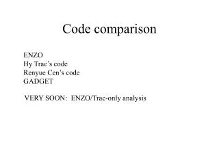

Code comparison
E N D
Presentation Transcript
Code comparison ENZO Hy Trac’s code Renyue Cen’s code GADGET VERY SOON: ENZO/Trac-only analysis
Code comparison Blue: Cen Black: Trac Denominator: ENZO
Thermal histories Red: Cen Black: Trac Green: ENZO Blue: GADGET
Dependence of Cosmology result On simulation type (in analysis, we marginalized over the differences between 3 Cen simulations)
Mean absorption Direct PCA analysis and power spectrum analysis of SDSS data agree, and agree with HIRES results.
PCA analysis of QSO spectra Evolution of mean flux consistent with external constraints No feature at z=3.2
Ly-alpha forest SDSS quasar spectrum Cen simulation of the IGM (neutral hydrogen) z = 3.7 quasar
Assumed cosmological parameters True cosmological parameters Theory (simulations) Observations Statistics (power spectrum) Statistics (power spectrum) Compare (chi^2)
Scales of various LSS probes The Ly forest is great for determining the running of the spectral index, , because it extends our knowledge to small scales We only report an amplitude and slope no band powers (out of date figure by Max Tegmark)
Constraints in the natural LyaF plane from WMAP, minimal model, with and without running
No evidence for departure from scale-invariance n=1, dn/dlnk=0 3-fold reduction in errors on alpha_s Very large running ruled out
Pre-SDSS LyaF power spectrum measurements: • Croft et al. (1999) 19 low resolution spectra • McDonald et al. (2000) 8 Keck/HIRES spectra • Croft et al. (2002) 30 Keck/HIRES, 23 Keck/LRIS spectra • Kim et al. (2004) 27 VLT/UVES spectra
SDSS Data 3300 spectra with zqso>2.3 (DR3 has 5767) redshift distribution of quasars 1.4 million pixels in the forest redshift distribution of Ly forest pixels
Measured Power • 2(k) = π-1 k P(k) (0.01 s/km ~ 1 h/Mpc) • Colors correspond to redshift bins centered at z = 2.2, 2.4, …, 4.2 (from bottom to top) • 1041<rest<1185 Å • Computed using optimal weighting • Noise subtraction • Resolution correction • Background subtraction using regions with rest>1268 Å • Error bars from bootstrap resampling • Code tested on semi-realistic mock spectra • HIRES/VLT data probes smaller scales • Computationally only modestly challenging
Fractional Errors • Lines connect the fractional errors on PF(k) points • Equivalent to an overall amplitude measurement to +-0.6% • Logarithmic slope measurement to +-0.006
Noise Power • Ratio of noise power to signal power • Important to subtract accurately, especially on small scales (in the future we won’t need noise subtraction because can cross-correlate multiple exposures)
Residual Noise Power • Power in measured from differences between exposures of the same quasar • Should be zero • Actually consistent with a 16% underestimate of the noise subtraction term • Probably due to error in initial “gain”, maybe some sky subtraction noise
Bootstrap error estimates • Bootstrap resampling by quasar • Tested using mock spectra • Diagonal errors reasonably close to Gaussian
Error Correlations Inverted window function Un-inverted window function
Resolution test • W2(k R) = exp[-(k R)2] I measured the power in the sky spectra near the 5577 Å line (a delta function), and divided by the resolution estimate.
Background Contamination • The top set of lines shows the Ly forest power • The bottom set of lines shows the power in the region 1268<rest<1380Å
Background Fraction • Probably mostly metals (CIV), but not all. • Error bars starting at zero show error on the forest power.
Difference Between two Background Estimates • Difference in power between the regions 1268<rest<1380Å and 1409<rest<1523Å
Our Simulations • Predict PF(k) using simulations of a large grid in parameter space and compare directly to the observed PF(k). • Allow general relation PF(k) = f[PL(k)] (but only amplitude, slope, and curvature of PL(k)], no band powers). • IGM gas in ionization equilibrium with a not necessarily homogeneous UV background (still assuming homogeneous reionization). • Assume IGM not arbitrarily badly disturbed by feedback from galaxies (but allow for some winds). • Fully hydrodynamic simulations near the best-fit cosmological model are used to calibrate approximate hydro-PM simulations which are used to explore parameter space. • Marginalize over temperature density relation parameters, T=T0(1+)-1, mean absorption level, reionization history, etc.
Nuisance parameters Errors +-0.01 on both parameters if modeling uncertainty is ignored: Noise/resolution Mean absorption Temperature-density Damping wings SiIII UV background fluctuations Galactic winds reionization
Best fitted model • 2 ≈ 185.6 for 161 d.o.f. • A single model fits the data over a wide range of redshift and scale • Wiggles from SiIII-Ly cross-correlation • Helped some by HIRES data
Theory now includes: • Rudimentary galactic superwinds (known to exist in starburst galaxies and LBGs) • Ionizing background fluctuations from quasars • Damped and lyman limit systems, which are not well modeled in simulations
Fluctuations in the ionizing background • Place quasars with a given luminosity function and lifetime in dark matter halos in a large (320 Mpc/h - Bode & Ostriker) N-body simulation (also try galaxies). • Compute the radiation field produced by the sources, including attenuation by the IGM. (Uros Seljak) • Fluctuations can be large at high redshift where the attenuation length is short.
Fluctuations in ionizing background Attenuation length is rapidly decreasing with redshift, so effect can be large at z>4, negligible at lower redshifts
Fluctuations in ionizing background Correlation of galaxies with density leads to coherent fluctions - suppression of power
Galactic winds heat IGM to 100,000K and pollute IGM with metals Temperature maps No wind wind Cen, Nagamine, Ostriker 2004
Neutral hydrogen maps show much less effect No wind wind
Strong wind versus no wind simulations Winds have no effect after simulations have been adjusted for temperature change This is not conclusive and more work is needed to investigate other possible wind models
Damped and lyman limit systems • When density of hydrogen is high photons get absorbed and do not ionize hydrogen (self-shielding) • Simulations generally cannot simulate this accurately • We have measurements of the number density of these systems as a function of column density and redshift • We place these systems into densest regions of simulations • Damping wings (Lorenzians) wipe out a large section of the spectrum • This adds long wavelength power, removing it makes spectrum bluer • Important effect which was not previously estimated
Can determine power law slope of the growth factor to 0.1 Mandelbaum etal 2003
Comparison with theory (first try) • Curves from simulations • Fitted parameters: Amplitude and slope of the primordial power spectrum, mean absorption level, and temperature-density relation for the gas • 2 ≈ 192 for 106 degrees of freedom!
SiIII-Ly cross-correlation bump • SiIII absorbs at 1207 Å, corresponding to a velocity offset 2271 km/s • Vertical line at 2271 km/s • No other obvious bumps out to about 7000 km/s • Dashed line shows 0.04 F(v-2271 km/s)/ F(0)
Best fitted model • 2 ≈ 185.6 for 161 d.o.f. • A single model fits the data over a wide range of redshift and scale • Wiggles from SiIII-Ly cross-correlation • Helped some by HIRES data
Self calibration Errors +-0.01 on both parameters if modeling uncertainty is ignored: Noise/resolution Mean absorption Temperature-density Damping wings SiIII UV background fluctuations Winds reionization
Model uncertainties If potential systematic errors were ignored, errors would be a factor of 5 smaller!
Model uncertainties Uncertainties in the estimate of the noise and resolution of the SDSS data are allowed for
Model uncertainties Evolving cross-correlation between Lyman-alpha and SiIII absorption is included in the model (no change at this point)
Model uncertainties An evolving relation between temperature and density is included in the model (dotted line shows previous case)