Lecture 4 Image Enhancement in the Frequency Domain

1. Lecture 4 Image Enhancement in the Frequency Domain Cosimo Distante

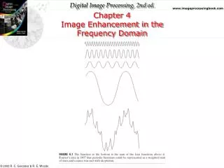
2. Any function that periodically repeats itself can be expressed as the sum of sines and/or cosines of different frequencies, each multiplied by a different coefficient (Fourier series). Even functions that are not periodic (but whose area under the curve is finite) can be expressed as the integral of sines and/or cosines multiplied by a weighting function (Fourier transform). Background

3. The frequency domain refers to the plane of the two dimensional discrete Fourier transform of an image. The purpose of the Fourier transform is to represent a signal as a linear combination of sinusoidal signals of various frequencies. Background

4. Introduction to the Fourier Transform and the Frequency Domain • The one-dimensional Fourier transform and its inverse • Fourier transform (continuous case) • Inverse Fourier transform: • The two-dimensional Fourier transform and its inverse • Fourier transform (continuous case) • Inverse Fourier transform:

5. Introduction to the Fourier Transform and the Frequency Domain • The one-dimensional Fourier transform and its inverse • Fourier transform (discrete case) DTC • Inverse Fourier transform:

6. Introduction to the Fourier Transform and the Frequency Domain • Since and the fact then discrete Fourier transform can be redefined • Frequency (time) domain: the domain (values of u) over which the values of F(u) range; because u determines the frequency of the components of the transform. • Frequency (time) component: each of the M terms of F(u).

7. Introduction to the Fourier Transform and the Frequency Domain • F(u) can be expressed in polar coordinates: • R(u): the real part of F(u) • I(u): the imaginary part of F(u) • Power spectrum:

8. The One-Dimensional Fourier Transform Example

9. The transform of a constant function is a DC value only. The transform of a delta function is a constant. The One-Dimensional Fourier Transform Some Examples

10. The transform of an infinite train of delta functions spaced by T is an infinite train of delta functions spaced by 1/T. The transform of a cosine function is a positive delta at the appropriate positive and negative frequency. The One-Dimensional Fourier Transform Some Examples

11. The transform of a sin function is a negative complex delta function at the appropriate positive frequency and a negative complex delta at the appropriate negative frequency. The transform of a square pulse is a sinc function. The One-Dimensional Fourier Transform Some Examples

12. Introduction to the Fourier Transform and the Frequency Domain • The two-dimensional Fourier transform and its inverse • Fourier transform (discrete case) DTC • Inverse Fourier transform: • u, v : the transform or frequency variables • x, y : the spatial or image variables

13. Introduction to the Fourier Transform and the Frequency Domain • We define the Fourier spectrum, phase angle, and power spectrum as follows: • R(u,v): the real part of F(u,v) • I(u,v): the imaginary part of F(u,v)

14. Introduction to the Fourier Transform and the Frequency Domain • Some properties of Fourier transform:

15. (a)f(x,y) (b)F(u,y) (c)F(u,v) The Two-Dimensional DFT and Its Inverse • The 2D DFT F(u,v) can be obtained by • taking the 1D DFT of every row of image f(x,y), F(u,y), • taking the 1D DFT of every column of F(u,y)

16. The Two-Dimensional DFT and Its Inverse shift

17. The Two-Dimensional DFT and Its Inverse

18. The Property of Two-Dimensional DFT Rotation DFT DFT

19. The Property of Two-Dimensional DFT Linear Combination A DFT B DFT 0.25 * A + 0.75 * B DFT

20. The Property of Two-Dimensional DFT Expansion A DFT B DFT Expanding the original image by a factor of n (n=2), filling the empty new values with zeros, results in the same DFT.

21. Two-Dimensional DFT with Different Functions Its DFT Sine wave Rectangle Its DFT

22. Two-Dimensional DFT with Different Functions Its DFT 2D Gaussian function Impulses Its DFT

23. Filtering in the Frequency Domain

24. Basics of Filtering in the Frequency Domain

25. Some Basic Filters and Their Functions • Multiply all values of F(u,v) by the filter function (notch filter): • All this filter would do is set F(0,0) to zero (force the average value of an image to zero) and leave all frequency components of the Fourier transform untouched.

26. Some Basic Filters and Their Functions Lowpass filter Highpass filter

27. Some Basic Filters and Their Functions

28. Correspondence between Filtering in the Spatial and Frequency Domain • Convolution theorem: • The discrete convolution of two functions f(x,y) and h(x,y) of size M×N is defined as • Let F(u,v) and H(u,v) denote the Fourier transforms of f(x,y) and h(x,y), then Eq. (4.2-31) Eq. (4.2-32)

29. Correspondence between Filtering in the Spatial and Frequency Domain • :an impulse function of strength A, located at coordinates (x0,y0) where : a unit impulse located at the origin • The Fourier transform of a unit impulse at the origin (Eq. (4.2-35)) :

30. Correspondence between Filtering in the Spatial and Frequency Domain • Let , then the convolution (Eq. (4.2-36)) • Combine Eqs. (4.2-35) (4.2-36) with Eq. (4.2-31), we obtain

31. Correspondence between Filtering in the Spatial and Frequency Domain • Let H(u) denote a frequency domain, Gaussian filter function given the equation where : the standard deviation of the Gaussian curve. • The corresponding filter in the spatial domain is • Note: Both the forward and inverse Fourier transforms of a Gaussian function are real Gaussian functions.

32. Correspondence between Filtering in the Spatial and Frequency Domain

33. Correspondence between Filtering in the Spatial and Frequency Domain • One very useful property of the Gaussian function is that both it and its Fourier transform are real valued; there are no complex values associated with them. • In addition, the values are always positive. So, if we convolve an image with a Gaussian function, there will never be any negative output values to deal with. • There is also an important relationship between the widths of a Gaussian function and its Fourier transform. If we make the width of the function smaller, the width of the Fourier transform gets larger. This is controlled by the variance parameter 2 in the equations. • These properties make the Gaussian filter very useful for lowpass filtering an image. The amount of blur is controlled by 2. It can be implemented in either the spatial or frequency domain. • Other filters besides lowpass can also be implemented by using two different sized Gaussian functions.

34. Smoothing Frequency-Domain Filters • The basic model for filtering in the frequency domain where F(u,v): the Fourier transform of the image to be smoothed H(u,v): a filter transfer function • Smoothing is fundamentally a lowpass operation in the frequency domain. • There are several standard forms of lowpass filters (LPF). • Ideal lowpass filter • Butterworth lowpass filter • Gaussian lowpass filter

35. Ideal Lowpass Filters (ILPFs) • The simplest lowpass filter is a filter that “cuts off” all high-frequency components of the Fourier transform that are at a distance greater than a specified distance D0 from the origin of the transform. • The transfer function of an ideal lowpass filter where D(u,v) : the distance from point (u,v) to the center of ther frequency rectangle

36. Ideal Lowpass Filters (ILPFs)

37. Ideal Lowpass Filters (ILPFs)

38. Ideal Lowpass Filters

39. Butterworth Lowpass Filters (BLPFs) With order n

40. Butterworth Lowpass Filters (BLPFs) n=2 D0=5,15,30,80,and 230

41. Butterworth Lowpass Filters (BLPFs) Spatial Representation n=1 n=2 n=5 n=20

42. Gaussian Lowpass Filters (FLPFs)

43. Gaussian Lowpass Filters (FLPFs) D0=5,15,30,80,and 230

44. Additional Examples of Lowpass Filtering

45. Additional Examples of Lowpass Filtering

46. Sharpening Frequency Domain Filter Ideal highpass filter Butterworth highpass filter Gaussian highpass filter

47. Highpass Filters Spatial Representations

48. Ideal Highpass Filters

49. Butterworth Highpass Filters

50. Gaussian Highpass Filters