Adaptive Networks
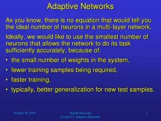
Adaptive Networks. As you know, there is no equation that would tell you the ideal number of neurons in a multi-layer network. Ideally, we would like to use the smallest number of neurons that allows the network to do its task sufficiently accurately, because of:

Adaptive Networks
E N D
Presentation Transcript
Adaptive Networks • As you know, there is no equation that would tell you the ideal number of neurons in a multi-layer network. • Ideally, we would like to use the smallest number of neurons that allows the network to do its task sufficiently accurately, because of: • the small number of weights in the system, • fewer training samples being required, • faster training, • typically, better generalization for new test samples. Neural Networks Lecture 13: Adaptive Networks
Adaptive Networks • So far, we have determined the number of hidden-layer units in BPNs by “trial and error.” • However, there are algorithmic approaches for adapting the size of a network to a given task. • Some techniques start with a large network and then iteratively prune connections and nodes that contribute little to the network function. • Other methods start with a minimal network and then add connections and nodes until the network reaches a given performance level. • Finally, there are algorithms that combine these “pruning” and “growing” approaches. Neural Networks Lecture 13: Adaptive Networks
Cascade Correlation • None of these algorithms are guaranteed to produce “ideal” networks. • (It is not even clear how to define an “ideal” network.) • However, numerous algorithms exist that have been shown to yield good results for most applications. • We will take a look at one such algorithm named “cascade correlation.” • It is of the “network growing” type and can be used to build multi-layer networks of adequate size. • However, these networks are not strictly feed-forward in a level-by-level manner. Neural Networks Lecture 13: Adaptive Networks
Refresher: Covariance and Correlation • For a dataset (xi, yi) with i = 1, …, n the covariance is: y y y y y y x x x x x x cov(x,y) > 0 cov(x,y) ≈ 0 cov(x,y) < 0 Neural Networks Lecture 13: Adaptive Networks
Refresher: Covariance and Correlation • Covariance tells us something about the strength and direction (directly vs. inversely proportional) of the linear relationship between x and y. • For many applications, it is useful to normalize this variable so that it ranges from -1 to 1. • The result is the correlation coefficient r, which for a dataset (xi, yi) with i = 1, …, n is given by: Neural Networks Lecture 13: Adaptive Networks
Refresher: Covariance and Correlation 0 < r < 1 r ≈ 0 -1 < r < 0 y y y y y y x x x x x x r = 1 r = -1 r undef’d Neural Networks Lecture 13: Adaptive Networks
Refresher: Covariance and Correlation • In the case of high (close to 1) or low (close to -1) correlation coefficients, we can use one variable as a predictor of the other one. • To quantify the linear relationship between the two variables, we can use linear regression: y regression line x Neural Networks Lecture 13: Adaptive Networks
Cascade Correlation • Now let us return to the cascade correlation algorithm. • We start with a minimal network consisting of only the input neurons (one of them should be a constant offset = 1) and the output neurons, completely connected as usual. • The output neurons (and later the hidden neurons) typically use output functions that can also produce negative outputs; e.g., we can subtract 0.5 from our sigmoid function for a (-0.5, 0.5) output range. • Then we successively add hidden-layer neurons and train them to reduce the network error step by step: Neural Networks Lecture 13: Adaptive Networks
Cascade Correlation Output node o1 • Input nodes Solid connections are being modified x1 x2 x3 Neural Networks Lecture 13: Adaptive Networks
Cascade Correlation Output node o1 • Input nodes Solid connections are being modified First hidden node x1 x2 x3 Neural Networks Lecture 13: Adaptive Networks
Cascade Correlation Output node o1 Secondhidden node • Input nodes Solid connections are being modified First hidden node x1 x2 x3 Neural Networks Lecture 13: Adaptive Networks
Cascade Correlation • Weights to each new hidden node are trained to maximize the covariance of the node’s output with the current network error. • Covariance: : vector of weights to the new node : output of the new node to p-th input sample : error of k-th output node for p-th input sample before the new node is added : averages over the training set Neural Networks Lecture 13: Adaptive Networks