Input-output Controllability Analysis
Input-output Controllability Analysis. Idea: Find out how well the process can be controlled - without having to design a specific controller. Reference: S . Skogestad, ``A procedure for SISO controllability analysis - with application to design of pH neutralization processes'',

Input-output Controllability Analysis
E N D
Presentation Transcript
Input-output Controllability Analysis Idea: Find out how well the process can be controlled - without having to design a specific controller Reference: S. Skogestad, ``A procedure for SISO controllability analysis - with application to design of pH neutralization processes'', Comp.Chem.Engng., 20, 373-386, 1996.
Two main rules. • Rule 1: speed of response • Fast response required to reject large disturbance • BUT: Response time is limited by effective time delay • Rule 2: Input constraints • Also: Large disturbance rejection may give input saturation
Ideal controller inverts the plant • y = g(s)u + d • Ideal controller inverts the plant g(s): • Think feedforward, u = cff(s) (ys-d) • Perfect control: want y=ys)cff = 1/g(s) = g-1 Limitations on perfect control: Inverse cannot always be realized: • Input saturation , |u| > |umax| • Time delay, g=e-µs . • g-1= eµs = prediction (not possible) • Solution: Omit • Inverse response, g = -Ts+1. • g-1 = 1/(-Ts+1) = unstable (not possible as u will be unbounded) • Solution: Omit • More poles than zeros, g = 1/(¿ s+1), • g-1 = ¿ s + 1 = pure differentiation (not possible as u will be unbounded). • Solution: Replace by: (¿s + 1)/(¿c+1) where ¿c< ¿ is a tuning parameter • Example. g(s) = 5 (-0.5s+1) e-2s / (3s+1). • Realizable inverse (feedforward): 0.2 (3s+1)/(¿c+1). E.g. choose ¿c=0.5 • So we know what limits us from having perfect control • Same limitations apply to feedback control • Controllability analysis: Want to find out what these limitations imply in terms of “acceptable control”, |y-ys|·ymax
SCALED MODEL MAIN REASON FOR CONTROL: DISTURBANCES! Need control up to frequency !d where |Gd|=1 -> Need !c > !d (!c is frequency where |L|=1) Proof: y = Gd/(1+L)d, where L = GC (“llop”) Worst-case is |d|=1. Want |y| <1, so want |Gd|<|1+L| ¼ |L| (approximation holds at low frequencies where |L| is large). Conclusion: Need |L|>|Gd| at frequencies where |Gd|>1 Gd !c L=gc !d Note: !B=!c=1/¿c
Rules for speed of response (assuming control with integral action) • Define !c=1/¿c = closed-loop bandwidth = where |gc| is 1 • Rule 1a: Need !c >!d (¿c < 1/!d) • Where !d is frequency where |g’d|=1. • Rule 1 is for typical case where |g’d| is highest at low frequencies • Rule 1b: Need !c < 1/µ (¿c > µ) • Where µ is effective time delay • Rule 1c: Need !c > p (¿c < 1/p) • Where p is unstable pole, g(s) =k/(s-p)… This order is OK according to rule 1: !d p 1/µ ! !c must be in this range
SCALED MODEL 3 10 2 10 1 10 0 10 -1 10 -2 10 -3 -2 -1 0 1 10 10 10 10 10 EXAMPLE |G| |Gd| !d=0.9 s=tf('s') g = 500/((50*s+1)*(10*s+1)) gd = 9/(10*s+1) w = logspace(-3,1,1000); [mag,phase]=bode(g,w); [magd,phased]=bode(gd,w); loglog(w,mag(:),'blue',w,magd(:),'red',w,1,'black'), grid on PI-control: 1/µ = 1/5 = 0.2 PID-control: 1/µ = 1/0 = 1
SCALED MODEL 6 5 4 3 2 1 0 0 50 100 150 200 250 300 350 400 450 500 PI control not acceptable* s=tf('s') g = 500/((50*s+1)*(10*s+1)) gd = 9/(10*s+1) % SIMC-PI with tauc=theta=5 Kc=(1/500)*(55/(5+5)); taui=55; taud=0; y § 1 *As expected since need !c > !d= 0.9, but can only achieve !c<1/µ = 1/5 = 0.2
SCALED MODEL 2 1.5 1 0.5 0 -0.5 -1 0 50 100 150 200 250 300 350 400 450 500 PID control acceptable: y and u are § 1 y u g = 500/((50*s+1)*(10*s+1)) gd = 9/(10*s+1) %SIMC-PID (cascade form) with tauc=wd=1: Kc=(1/500)*(50/(1+0)); taui=50; taud=10;
If process is not controllable: Need to change the design • For example, dampen disturbance by adding buffer tank: Level control unimportant, but need good mixing Level control is NOT tight -> level varies Integral action is not recommended for averaging level control
SCALED MODEL Problem 1
SCALED MODEL Problem 2
SCALED MODEL Problem 3 -
SCALED MODEL Problem 4 g = 200/((20*s+1)*(10*s+1)*(s+1)) gd = 4/((3*s+1)*(s+1)^3) Kc=(1/200)*20/1,taui=20,taud=10.5
SCALED MODEL Problem 5 -
SCALED MODEL Problem 6 pH-Neutralization. y = cH+ - cOH- (want=0§10-6mol/l,pH=7§1) u = qbase(cOH-=10mol/l, pH=15) d = qacid (cH+ =10mol/l, pH=-1) Using tanks in series, Acid and base in tank 1. Scaled model: kd = 2.5e6 Each tank: ¿ = 1000s Control: µ = 10s (meas. delay for pH) Problem: How many tanks? |Gd| n=1 n=2 n=3 ! [rad/s] Reference for more applications of controllability analysis: Chapter 5 in book by Skogestad and Postlethwaite (2005)
Control system • 3 tanks: Neutralization (base addition) only in tank 1 gives large effective delay (>> 10s) because of tank dynamics in g(s) • Suggested solution is to add (a little) base also in the other tanks: pH 2 pH 5