Download
1 / 77
770 likes | 884 Vues
Introduction to Geographic Information Systems Spring 2013 (INF 385T-28437) Dr. David Arctur Lecturer, Research Fellow University of Texas at Austin Lecture 7 Feb 21, 2013 Spatial Data and Geoprocessing. Outline. Bolstad , Ch 5, 6, 7: Data Sources, cont’d

E N D
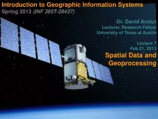
Introduction to Geographic Information Systems Spring 2013 (INF 385T-28437) Dr. David Arctur Lecturer, Research Fellow University of Texas at Austin Lecture 7 Feb 21, 2013 Spatial Data and Geoprocessing
Outline INF385T(28437) – Spring 2013 – Lecture 7 • Bolstad, Ch 5, 6, 7: Data Sources, cont’d • GPS, Aerial/Satellite Imagery, Digital Data • Gorr & Kurland, Ch 8: Geoprocessing • Attribute extraction • Feature location extraction • Location proximities • Geoprocessing tools • Model builder
Lecture 7 More on Data sources: GPS, Imagery, digital INF385T(28437) – Spring 2013 – Lecture 7
Measuring location & data INF385T(28437) – Spring 2013 – Lecture 7 • Three main approaches, many technologies: • In situ: make field observations on site • Stream flow & other gauges, GPS location • Remote sensing: observe from a distance • Aerial photos, satellite sensors, LiDAR • Model results: products derived from working on other products
Global Navigation Systems Bolstad, p.184 INF385T(28437) – Spring 2013 – Lecture 7 Aka, Global Positioning Systems (GPS) Global Navigation Satellite Systems (GNSS) Uses WGS84 for coordinate reference system
GPS Ranging: get 4+ Bolstad, p.189 INF385T(28437) – Spring 2013 – Lecture 7
GPS Errors due to receiver sensitivity PDOP: Positional Dilution of Precision (see Bolstad, p.192) INF385T(28437) – Spring 2013 – Lecture 7
GPS: Differential Correction Bolstad, p.195 INF385T(28437) – Spring 2013 – Lecture 7 Depends on having GPS receivers with precisely known location Differential correction can be applied in real-time or calculated later
Remote Sensing Bolstad, chapter 6 INF385T(28437) – Spring 2013 – Lecture 7 Aerial photography Satellite multispectral / hyperspectral LiDAR – Light Detection and Ranging Sensor webs
Industrial Process Monitor Sensor Webs Automobile as Sensor Probe Environmental Monitor Temp Sensor Traffic, Bridge Monitoring Stored Sensor Data Airborne Imaging Device Webcam Strain Gauge Health Monitor Satellite-borne Imaging Device INF385T(28437) – Spring 2013 – Lecture 7 • Sensors connected to and discoverable on Web • Sensors have position & generate observations • Sensor descriptions available • Services to task and access sensors • Local, regional, national scalability • Enabling the Enterprise Source: OGC
LiDAR – Laser-based imagery Bolstad, p.260 INF385T(28437) – Spring 2013 – Lecture 7 Hi-resolution topography Can separate forest cover from ground layer
LiDAR point clouds Bolstad, p.261 INF385T(28437) – Spring 2013 – Lecture 7
LiDAR Applications Source: Wikipedia INF385T(28437) – Spring 2013 – Lecture 7 Agriculture yields Biology, conservation Archaeology beneath forest canopy Geology, soil science 3D cave maps, hi-resolution beach topography Meteorology, law enforcement, robotics Adaptive cruise control (autos)
Spatial Processing INF385T(28437) – Spring 2013 – Lecture 7 Attribute extraction Feature location extraction Location proximities Geoprocessing tools Model builder
Lecture 7 Spatial Processing: Attribute extraction INF385T(28437) – Spring 2013 – Lecture 7
Attribute query extraction INF385T(28437) – Spring 2013 – Lecture 7 You have tracts for an entire state, but want tracts for one county only
Attribute query extraction INF385T(28437) – Spring 2013 – Lecture 7 • Select tracts by County FIPS ID • Cook County = 031
Attribute query extraction INF385T(28437) – Spring 2013 – Lecture 7 Cook County tractsselected Export to new featureclass or shapefile
Export selected features • Right-click to export selected features INF385T(28437) – Spring 2013 – Lecture 7
Add new layer INF385T(28437) – Spring 2013 – Lecture 7 Cook County tracts
Lecture 7 Feature location extraction INF385T(28437) – Spring 2013 – Lecture 7
Select by location INF385T(28437) – Spring 2013 – Lecture 7 Powerful function unique to GIS Identify spatial relationships between layers Finds features that are within another layer
Select by location INF385T(28437) – Spring 2013 – Lecture 7 • Have Cook County census tracts but want City of Chicago only • Can’t use Select By Attributes • No attribute for Chicago • Use “Municipality” layer • City Chicago is a municipality within Cook County
Select by location INF385T(28437) – Spring 2013 – Lecture 7 Select “Chicago” from municipalities layer
Select by location • Selection, Select By location INF385T(28437) – Spring 2013 – Lecture 7
Export selected features INF385T(28437) – Spring 2013 – Lecture 7
Lecture 7 location proximities INF385T(28437) – Spring 2013 – Lecture 7
Points near polygons INF385T(28437) – Spring 2013 – Lecture 7 Health officials want to know polluting companies near water features
Points near points INF385T(28437) – Spring 2013 – Lecture 7 School officials want to know what schools are near polluting companies
Polygons intersecting lines INF385T(28437) – Spring 2013 – Lecture 7 Transportation planner wants to know what neighborhoods are affected by construction project on major highway
Lines intersecting polygons INF385T(28437) – Spring 2013 – Lecture 7 Public works official wants to know what streets or sidewalks will be affected by potential floods
Polygons completely within polygons INF385T(28437) – Spring 2013 – Lecture 7 City planners want to know what buildings are completely within a zoning area.
Lecture 7 Geoprocessing tools INF385T(28437) – Spring 2013 – Lecture 7
Geoprocessing overview INF385T(28437) – Spring 2013 – Lecture 7 GIS operations to manipulate data Typically take input data sets, manipulate, and produce output data sets Often use multiple data sets
Geoprocessingenablesdecisions Assess Wildfire Danger GeoprocessingWorkflow To create derived & value-added products Decision Support Client Internet Base map from NASA Data Pool Coordinate transformation Classify fire areas from aerials Overlay and buffer Roads layer … Data Servers (web services) INF385T(28437) – Spring 2013 – Lecture 7 Source: OGC
Common geoprocessing tools INF385T(28437) – Spring 2013 – Lecture 7 • Analysis • Extract – Clip • Overlay – intersect and union • Data management • Generalization - dissolve • General • Append • Merge
Finding the tools INF385T(28437) – Spring 2013 – Lecture 7 • Geoprocessing menu (slight differences between 10.0 and 10.1)
Finding the tools INF385T(28437) – Spring 2013 – Lecture 7 ArcToolbox
Finding the tools INF385T(28437) – Spring 2013 – Lecture 7 Search window
Clip Clip features (Central Business District) Input features (streets) Output features (CBD streets) INF385T(28437) – Spring 2013 – Lecture 7 Acts like a “cookie cutter” to create a subset of features
Clip INF385T(28437) – Spring 2013 – Lecture 7
Clip vs. select-by-location INF385T(28437) – Spring 2013 – Lecture 7 • Clip • Clean edges • Looks good • Select by location • Dangling edges • Better for geocoding
Dissolve INF385T(28437) – Spring 2013 – Lecture 7 Combines adjacent polygons to create new, larger polygons Uses common field value to remove interior lines within each polygon, forming the new polygons Aggregate (sums) data while dissolving
Dissolve INF385T(28437) – Spring 2013 – Lecture 7 • Create regions using U.S. states • Use SUB_REGION field to dissolve • Sum population
Dissolve Statistics Fields (optional) (may not be initially visible,scroll down to see) INF385T(28437) – Spring 2013 – Lecture 7
Dissolve results INF385T(28437) – Spring 2013 – Lecture 7 States dissolved to form regions Population summed for each region
Append INF385T(28437) – Spring 2013 – Lecture 7 • Appends one or more data sets into an existing data set • Features must be of the same type • Input datasets may overlap one another and/or the target dataset • TEST option: field definitions of the feature classes must be the same and in the same order for all appended features • NO TEST option: Input features schemasdo not have to match the target feature classes' schema
Append • DuPage and Cook County are combining public works and need a new single street centerline file. INF385T(28437) – Spring 2013 – Lecture 7
Append INF385T(28437) – Spring 2013 – Lecture 7 Append will addDuPage streets to Cook County streets
Resultant layer • One street layer (Cook County) with all records and field items INF385T(28437) – Spring 2013 – Lecture 7