Noise in Imaging Technology

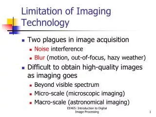
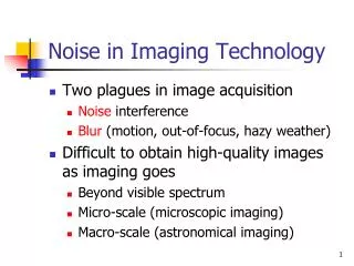
Noise in Imaging Technology • Two plagues in image acquisition • Noise interference • Blur (motion, out-of-focus, hazy weather) • Difficult to obtain high-quality images as imaging goes • Beyond visible spectrum • Micro-scale (microscopic imaging) • Macro-scale (astronomical imaging)

What is Noise? • noise means any unwanted signal • One person’s signal is another one’s noise • Noise is not always random and randomness is an artificial term • Noise is not always bad.

Stochastic Resonance no noise heavy noise light noise

Image Denoising • Where does noise come from? • Sensor (e.g., thermal or electrical interference) • Environmental conditions (rain, snow etc.) • Why do we want to denoise? • Visually unpleasant • Bad for compression • Bad for analysis

Noisy Image Examples thermal imaging electrical interference physical interference ultrasound imaging

Noise Removal Techniques Linear filtering Nonlinear filtering Recall Linear system

Image Denoising • Introduction • Impulse noise removal • Median filtering • Additive white Gaussian noise removal • 2D convolution and DFT • Periodic noise removal • Band-rejection and Notch filter

Impulse Noise (salt-pepper Noise) Definition Each pixel in an image has the probability of p/2 (0<p<1) being contaminated by either a white dot (salt) or a black dot (pepper) with probability of p/2 noisy pixels with probability of p/2 clean pixels with probability of 1-p X: noise-free image, Y: noisy image Note: in some applications, noisy pixels are not simply black or white, which makes the impulse noise removal problem more difficult

Numerical Example P=0.1 128 128 128 128 128 128 128 128 128 128 128 128 128 128 128 128 128 128 128 128 128 128 128 128 128 128 128 128 128 128 128 128 128 128 128 128 128 128 128 128 128 128 128 128 128 128 128 128 128 128 128 128 128 128 128 128 128 128 128 128 128 128 128 128 128 128 128 128 128 128 128 128 128 128 128 128 128 128 128 128 128 128 128 128 128 128 128 128 128 128 128 128 128 128 128 128 128 128 128 128 128 128 255 0 128 128 128 128 128 128 128 128 128 128 0 128 128 128 128 0 128 128 128 128 128 128 128 128 128 128 128 128 0 128 128 128 128 128 128 128 128 128 128 128 128 128 128 128 128 128 128 128 128 128 128 128 128 128 128 128 128 128 128 128 128 128 128 128 128 128 0 128 128 128 128 255 128 128 128 128 128 128 128 128 128 128 128 128 128 255 128 128 128 128 128 128 128 255 128 128 X Y Noise level p=0.1 means that approximately 10% of pixels are contaminated by salt or pepper noise (highlighted by red color)

MATLAB Command >Y = IMNOISE(X,'salt & pepper',p) Notes:  The intensity of input images is assumed to be normalized to [0,1]. If X is double, you need to do normalization first, i.e., X=X/255;  The default value of p is 0.05 (i.e., 5 percent of pixels are contaminated)  imnoise function can produce other types of noise as well (you need to change the noise type ‘salt & pepper’)

Impulse Noise Removal Problem filtering algorithm denoised image ^ X ^ Can we make the denoised image X as close to the noise-free image X as possible? Noisy image Y

Median Operator • Given a sequence of numbers {y1,…,yN} • Mean: average of N numbers • Min: minimum of N numbers • Max: maximum of N numbers • Median: half-way of N numbers Example sorted

1D Median Filtering y(n) … … W=2T+1 MATLAB command: x=median(y(n-T:n+T)); Note: median operator is nonlinear

Numerical Example T=1: Boundary Padding

2D Median Filtering x(m,n) W: (2T+1)-by-(2T+1) window MATLAB command: x=medfilt2(y,[2*T+1,2*T+1]);

Numerical Example 225 225 225 226 226 226 226 226 225 225 255 226 226 226 225 226 226 226 225 226 0 226 226 255 255 226 225 0 226 226 226 226 225 255 0 225 226 226 226 255 255 225 224 226 226 0 225 226 226 225 225 226 255 226 226 228 226 226 225 226 226 226 226 226 0 225 225 226 226 226 226 226 225 225 226 226 226 226 226 226 225 226 226 226 226 226 226 226 226 226 225 225 226 226 226 226 225 225 225 225 226 226 226 226 225 225 225 226 226 226 226 226 225 225 225 226 226 226 226 226 226 226 226 226 226 226 226 226 ^ X Y Sorted: [0, 0, 0, 225, 225, 225, 226, 226, 226]

Image Example P=0.1 denoised image ^ Noisy image Y X 3-by-3 window

Idea of Improving Median Filtering • Can we get rid of impulse noise without affecting clean pixels? • Yes, if we know where the clean pixels are or equivalently where the noisy pixels are • How to detect noisy pixels? • They are black or white dots

Median Filtering with Noise Detection Noisy image Y Median filtering x=medfilt2(y,[2*T+1,2*T+1]); Noise detection C=(y==0)|(y==255); Obtain filtering results xx=c.*x+(1-c).*y;

Image Example noisy (p=0.2) clean with noise detection w/o noise detection

Additive White Gaussian Noise Definition Each pixel in an image is disturbed by a Gaussian random variable With zero mean and variance 2 X: noise-free image, Y: noisy image Note: unlike impulse noise situation, every pixel in the image contaminated by AWGN is noisy

Numerical Example 128 128 128 128 128 128 128 128 128 128 128 128 128 128 128 128 128 128 128 128 128 128 128 128 128 128 128 128 128 128 128 128 128 128 128 128 128 128 128 128 128 128 128 128 128 128 128 128 128 128 128 128 128 128 128 128 128 128 128 128 128 128 128 128 128 128 129 127 129 126 126 128 126 128 128 129 129 128 128 127 128 128 128 129 129 127 127 128 128 129 127 126 129 129 129 128 127 127 128 127 129 127 129 128 129 130 127 129 127 129 130 128 129 128 129 128 128 128 129 129 128 128 130 129 128 127 127 126 2=1 X Y

MATLAB Command >Y = IMNOISE(X,’gaussian',m,v) or >Y = X+m+randn(size(X))*v; rand() generates random numbers uniformly distributed over [0,1] Note: randn() generates random numbers observing Gaussian distribution N(0,1)

Image Denoising filtering algorithm denoised image ^ X Question: Why not use median filtering? Hint: the noise type has changed. Noisy image Y

1D Linear Filtering g(n) h(n) f(n) See review section Linear convolution - Linearity - Time-invariant property

Fourier Series forward inverse time-domain convolution frequency-domain multiplication Note that the input signal is a discrete sequence while its FT is a continuous function

Filter Examples |H(w)| Low-pass (LP) h(n)=[1,1] HP LP |h(w)|=2cos(w/2) High-pass (LP) h(n)=[1,-1] w |h(w)|=2sin(w/2)

2D Linear Filtering g(m,n) h(m,n) f(m,n) 2D convolution MATLAB function: C = CONV2(A, B)

2D Filtering=Two Sequential 1D Filtering Just as we have observed with 2D transform, 2D (separable) filtering can be viewed as two sequential 1D filtering operations: one along row direction and the other along column direction The order of filtering does not matter h1 : 1D filter

Fourier Series (2D case) spatial-domain convolution frequency-domain multiplication Note that the input signal is discrete while its FT is a continuous function

Filter Examples |h(w1,w2)| Low-pass (LP) h1(n)=[1,1] 1D |h1(w)|=2cos(w/2) h(n)=[1,1;1,1] 2D w2 |h(w1,w2)|=4cos(w1/2)cos(w2/2) w1

Image DFT Example choice 1: Y=fft2(X) Original ray image X

Image DFT Example (Con’t) choice 1: Y=fft2(X) choice 2: Y=fftshift(fft2(X)) Low-frequency at four corners Low-frequency at the center FFTSHIFT Shift zero-frequency component to center of spectrum.

Gaussian Filter FT MATLAB code: >h=fspecial(‘gaussian’, HSIZE,SIGMA);

Image Example denoised noisy denoised PSNR=20.2dB PSNR=24.4dB PSNR=22.8dB (=1) (=1.5) (=25) Matlab functions: imfilter, filter2

Gaussian Filter=Heat Diffusion Linear Heat Flow Equation: Isotropic diffusion: A Gaussian filter with zero mean and variance of t scale

Basic Idea of Nonlinear Diffusion* y I(x,y) x image I Diffusion should be anisotropic instead of isotropic image I viewed as a 3D surface (x,y,I(x,y))

Periodic Noise • Source: electrical or electromechanical interference during image acquistion • Characteristics • Spatially dependent • Periodic – easy to observe in frequency domain • Processing method • Suppressing noise component in frequency domain

Image Example spatial Frequency (note the four pairs of bright dots)

Band Rejection Filter w2 w1

Image Example After filtering Before filtering

Noise in Imaging Technology