Enhancing Phonetic Recognition with Conditional Random Fields (CRFs) in ASR Systems
This study explores the application of Conditional Random Fields (CRFs) for Automatic Speech Recognition (ASR) by implementing a system that performs first-pass phonetic recognition using discriminative training. We demonstrate that a CRF-based model surpasses Hidden Markov Models (HMMs) in phone recognition accuracy. With phonetic attributes defined according to the IPA chart and extracted using multi-layer perceptron classifiers trained on cepstral features, we outline the advantages of CRFs, including their ability to handle dependencies among features without the independence assumption found in HMMs.

Enhancing Phonetic Recognition with Conditional Random Fields (CRFs) in ASR Systems
E N D
Presentation Transcript
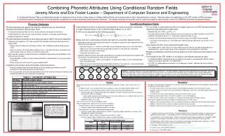
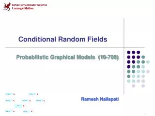
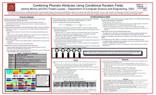
/sh/ /sh/ /iy/ /iy/ /iy/ X1 X2 X3 X4 X5 FIGURE 1: Spectrogram of the word /she/, shown with phonetic boundaries and corresponding phonetic attributes for each phone. Attributes are listed descending in the same order that they appear in Table 1. Combining Phonetic Attributes Using Conditional Random Fields Jeremy Morris and Eric Fosler-Lussier – Department of Computer Science and Engineering A Conditional Random Field is a mathematical model for sequences that is similar in many ways to a Hidden Markov Model, but is discriminative rather than generative in nature. Here we explore the application of the CRF model to ASR processing by building a system that performs first-pass phonetic recogintion using discriminatively trained phonetic attributes. This system achieves an accuracy level in a phone recognition task superior to that of an HMM that has been comparably trained. Conditional Random Fields • Phonetic Attributes • Phonetic attributes are defined via linguistic properties per the International Phonetics Association (IPA) phonetic chart • Consonants defined by their sonority, voicing, manner, and place of articulation • Vowels defined by their sonority, voicing, height, frontness, roundness and tenseness • Additional features for silence • Phonetic attributes extracted by multi-layer perceptron (MLP) neural net classifiers • Classifiers are trained on 12th order cepstral PLP and delta coefficients derived from the speech data • Speech data is broken up into frames of 25ms, with overlapping frames starting every 10ms • Input is a vector of PLP and delta coefficients for a nine frame window, centered on the current frame, with four frames of context on either side • Each classifier outputs a series of posterior probabilities representing the probability of the attribute given the data • One probability is output for each possible attribute for that classifier for any given frame of the data • These posteriors sum to one for a given classifier MLP • Classifiers were trained using phonetically transcribed corpus • Phonetic attribute labels were derived by using the attributes provided by the IPA description of the transcribed phone (See Figure 1) • For our purposes, all phones are assumed to have their canonical values for training, and attribute boundaries occur at phonetic boundaries • For our model, a state feature function is a single output from our MLP phonetic attribute classifiers associated with a single label • Example:sj(y,x,i) = MLPstop(xi)*δ(yi =/t/) • The state feature function above has the value of the output of our MLP classifier for the STOP attribute if the label at time i is /t/. Otherwise, it takes the value of zero. • Currently, transition feature functions do not use the output of the MLP neural networks • The value of the function is 1 if the label pair matches the pair defined for the function, 0 if it does not. • Each feature function has an associated weight value • This weight value is high when a non-zero feature function value is strongly associated with a particular label – giving a high value to the computation of the probability for that label • Weights are trained by maximizing the log likelihood of the training set with respect to the model • The strength of the CRF model is in its ability to use arbitrary features as input • In traditional HMMs, dependencies among features can lead to computationally difficult models – features are usually required to be independent • In a CRF, no independence assumption on the features is made. Features can have arbitrary dependencies. • A discriminative model of a sequence that attempts to model the posterior probability of a label sequence given a set of observed data (Lafferty, et. al, 2001) • A CRF can be described by the following equation: • Where each s is a state feature function and each t is a transition feature function • State feature functions associate observations in the data at a particular time segment with the label at that time segment • Described as s(y, x, i), where y is the label, x is the observed data, and i is the time frame. • Takes a non-zero value when the current label at frame i is the same as y and some observation in x holds for the frame i • Otherwise, the value is zero • Transition feature functions associate observations in the data at a particular time segment with the transition from the previous label into the current label • Described as t(y,y’,x,i), where y is the label, y’ is the previous label, x is the observed data, and i is the time frame • Takes a non-zero value when the current label at frame i is the same as y, the previous label is the same as y’, and some observation in xholds for the frame i FIGURE 2: Graphical model for a CRF phone labelling of the word /she/. The nodes labelled Xi indicate time frame observations for time frame i, while the nodes with phone labels indicate the phonetic labels for that time frame. Arcs between time frame observations and phone labels indicate dependencies between the observations and the identity of the phone (modelled using state feature functions and corresponding weights) while arcs between the phone label nodes indicate dependencies between neighboring phones (modelled using transition feature functions and corresponding weights). • Discussion • The CRF system trained on monophones has accuracy results that fall between that of the monophone trained Tandem and triphone trained Tandem systems. • The CRF system makes many fewer insertions (extra hypothesized phones) than the Tandem systems • The CRF system also makes many more deletions (missed phones where ones should be hypothesized) than the Tandem systems • The CRF system makes fewer hypotheses overall than either Tandem system • The precision measurement shows how often a hypothesis is a correct hypothesis • When the CRF system makes a hypothesis, it is correct more often than the Tandem systems • These results suggest some means to improve the performance of the CRF system: • Addition of new extracted attributes (such as a boundary detector) to incorporate into transition feature functions • Addition of a penalty factor on transition weights to generate more transitions • Addition of more contextual attributes into the state features to attempt to gain some level of triphonic context • Results • Phone-level accuracies of the CRF system were compared to a baseline Tandem system (Hermansky et. al, 2000) • A Tandem system uses the output of the neural networks as inputs to a Hidden Markov Model system • Tandem system was trained with both triphone label contexts and monophone label contexts • Triphone labels give a single left and right context phone to the label, allowing a finer level of context to be used when labels are assigned • In other words, the context for the phone /ae/ in the string of phones /k ae t/ is different from that in the string /k ae p/ since the right context is different • Monophone labels are a single • CRF system results are only for monophone labels • TABLE 2 (below) breaks down the results into three categories: • Phone Correctness: Was the correct phone hypothesized? • Number of correct labels divided by number of true labels • Phone Accuracy: Correctness penalized for overgeneration • Number of correct labels, penalized by the number of spuriously hypothesized labels (insertions), and divided by the number of true labels • Phone Precision: When a phone is hypothesized, how often is it right? • Number of correct labels, divided by the number of hypothesized labels • References • J. Lafferty, A. McCallum, and F. Pereira, “Conditional Random Fields: Probabilistic Models for Segmenting and Labelling Sequence Data”, in Proceedings of the 18th International Conference on Machine Learning, 2001. • H. Hermansky, D. Ellis, and S.Sharma, “Tandem connectionist feature stream extraction for conventional HMM systems”, in Proceedings of the IEEE Intl. Conf. on Acoustics, Speech, and Signal Processing, 2000. • M. Rajamanohar and E. Fosler-Lussier, “An evaluation of hierarchical articulatory feature detectors”, in IEEE Automatic Speech Recognition and Understanding Workshop, 2005. • S. Sarawagi, “CRF package for Java”, http://crf.sourceforge.net • D. Johnson et al. “ICSI QuickNet software”, http://www.icsi.berkely.edu/Speech/qn.html • S. Young et al. “HTK HMM software”, http://htk.eng.cam.ac.uk/

