Availability

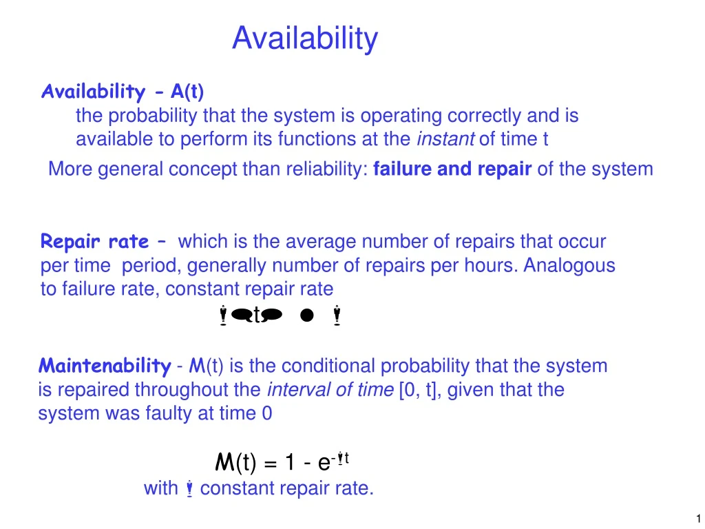
1. Availability Availability - A(t) the probability that the system is operating correctly and is available to perform its functions at the instant of time t More general concept than reliability: failure and repair of the system Repair rate – which is the average number of repairs that occur per time period, generally number of repairs per hours. Analogous to failure rate, constant repair rate m(t) = m Maintenability - M(t) is the conditional probability that the system is repaired throughout the interval of time [0, t], given that the system was faulty at time 0 M(t) = 1 - e-mt with m constant repair rate.

2. MTTR - The Mean Time To Repair is the average time required to repair the system. Analogous to MTTF, MTTR is expressed in terms of the repair rate: Failure events and repair events are not independent.

3. Model-based evaluation of dependability State-based models: Characterize the state of the system at time t: - identification of system states and changes of states The system goes from state to state as modules fail and repair. The state transitions are characterized by the probability of failure and the probability of repair - each state represents a distinct combination of failed and working modules - state transitions govern the changes of state that occur within a system

4. Model-based evaluation of dependability • - systems with arbitrary structures and complex dependencies can be modeled • - assumption of independent failures no longer necessary • used for both reliability and availability modeling • based on a Markov process, a special type of random process • Basic assumption underlying Markov models: • the system behavior at any time instant depends only on the current state(independent of past values)

5. N_failed(t) • Number of faulty components at time t (failures and repairs) 3 c1 repaired c1 fails 2 1 c2 fails c3 fails 0 c1 fails t N_failed(t) is a discrete function of a continuousparameter t Givendifferentfailure rate and repair rate, N_failed(t) functionisgoing to be different. Ifwehavelowerrepairrate, N_failed(t) will be higher in a stochasticsense.

6. Random variable Random variable a random variable X is a function from a sample space (Ω) to reals numbers Let us consider the random experiment of tossing a die. Let X be the random variable defined as the face you obtain Sample space Ω : faces of the die (1, 2, 3, 4, 5, 6) Real numbers S: 1, 2, 3, 4, 5, 6 Any element in the sample space Ω has a well defined probability distribution. The probability assigned to each output of the experiment is 1/6. If the set of values the variable can assume (S) is finite then X is a discrete random variable

7. Random variable Wedefine the probabilitydistributionfunctionof a discrete random variable: a mapping of allpossiblevalues of the random variable (S) to theircorresponfingprobabilities for the given sample spaceΩ f(x) = P(X=x) 1/6 for all i=1, …, 6 P(X=1)=1/6 f(x) = P(X=2)=1/6 0 otherwise……. An order relation can be defined on L. The probability of the following sets can be computed: P{X <= x0} for x0 in S Wedefine the cumulative distributionfunctionof X F(x0 ) = P {X <= x0} F is a non-decreasingfunction, if x1 <= x2 , then F(x1) <= F(x2) F(3) = P{X<=3} = P{X=1}+P{X=2}+P{X=3} = 1/6 +1/6+1/6 =1/2

8. Random variable Letusconsider the random experiment of the measuring the temperature in a region. Let X be the random variabledefinedas the temperature youobtain. Sample spaceΩ : Real numbers Real numbersS: Real numbers By definition, the probability of any real number is zero. The random variable can be infinitely divided into smaller parts such that the probability of selecting a real integer value x is zero. P(X=x) = 0 Probability is compiuted as: P(X <=x) P(X>=x) P(x1 <= x <= x2)

9. Random variable We define the probability density function: probability that a given output will occur at a given point An example of probability density function : Cumulative distribution function for a continuos random variable: which is the same as The probability density function can be computed by the cumulative distribution function if the derivative exists:

10. Random process Random process (or stochastic process) a collection of random variables {Xt } indexed by time The sequence of results of tossing a die can be expressed by a random process {Xt } with t = 0, 1, 2, 3. … (number of the throw) P[X0 = 4] = 1/6 P[X1 = 4 ] = 1/6 …. P[Xn = 4] = 1/6 Moreover P[Xn = 4 | Xn-1 = 2 ] = 1/6 In this case, the random variables are independent P[Xi = j] = 1/6 for all i and for all j Let S be the set of possible values of the random variable, these values are named states of the random variable. S is the state space of the random process.

11. Random processes: definitions State space S of a random process {Xt}: the set of all possible values the process can take S = {y: Xt = y, for some t} Discrete-state random process if the state space of random process is finite or countable (e.g., S={1, 2, 3, 4, 5, 6}) Continuous-state random processif the state space of random process is infinite or uncountable (e.g., S = the set of real numbers or an interval of real numbers ) Discrete-time random process all state transitions occur at fixed times (probabilities assigned to each transition) Continuous-time random process state transitions occur at random intervals (rates assigned to each transition)

12. Random processes The random process that reports the temperature in a region measured at each instant of time {Xt} S= { - <= x <= } T= { 0 <= t <= } continuos-space, continuos-time stochastic process Assume jobs enter the system randomly; after a waiting time, they are served and exit the system. Let {Xi} be the random process corresponding to the number of jobs in the system when jobs i arrives. {Xt} S={1,2, 3, …} T={1, 2, …} discrete-space, discrete-time stochastic process Let {Xi} be the random process corresponding to the number of jobs in the system at time t {Xt} S={0, 1,2, 3, …} T= { 0 <= t <= } discrete-space, continuous-time stochastic process

13. Random processes Type of dependency between random variables for different values of t Joint probability distribution function f(x0, x1, … , xn) = P {X0 =x0, X1=x1, …, Xn=xn } Cumulative distribution function for a joint probability distribution F(x0, x1, … , xn) = P {X0 <= x0, X1<=x1, …, Xn<=xn } In a general random process {Xt } the value of the random variable Xt+1 may depend on the values of all the previous random variables X0 X1 ............Xt.

14. Joint probability distribution function f(x0, x1, … , xn) = P {X0 = x0, X1=x1, …, Xn=xn } P {X0 = x0, X1=x1, …, Xn=xn }= P {Xn = xn | X0=x0, …, Xn-1=xn-1 } * P {X0=x0, …, Xn-1=xn-1 } = P {Xn-1= xn-1 | X0=x0 … Xn-2=xn-2 } * P {X0=x0, …, Xn-2=xn-2 } ……………………. f(x0, x1, … , xn) = P {Xn = xn | X0=x0, …, Xn-1=xn-1 } * P {Xn-1= xn-1 | X0=x0 … Xn-2=xn-2} * P {Xn-2= xn-2 | X0=x0 …. Xn-3=xn-3} * ……………… * P {X0=x0} Random process Sequence of tossing a die: P {X0=x0, X1=x1, …, Xn=xn }=P {X0=x0} * …. * P {Xn=xn }

15. Cumulative distribution function for a joint probability distribution F(x0, x1, … , xn) = P {X0 <= x0, X1<=x1, …, Xn<=xn } P {X0 <= x0, X1<=x1, …, Xn<=xn }= P {Xn <= xn | X0<=x0, …, Xn-1<=xn-1 } * P {X0<=x0, …, Xn-1<=xn-1 } = P {Xn-1<= xn-1 | X0<=x0 … Xn-2<=xn-2 } * P {X0<=x0, …, Xn-2<=xn-2 } … …………………. F(x0, x1, … , xn) = P {Xn <= xn | X0<=x0, …, Xn-1<=xn-1 } * P {Xn-1<= xn-1 | X0<=x0 … Xn-2<=xn-2} * P {Xn-2<= xn-2 | X0<=x0 …. Xn-3<=xn-3} * ……………… * P {X0<=x0}

16. Discrete-time Markov process Let be given {Xt } t = 0, 1, 2, … Basic assumption underlying a Markov process: the state of a process at time t+1 depends only on the state at time t, and is independent on any state before t. P{Xt+1 = j | X0 =x0, X1 =x1, …, Xt =it } = P{Xt+1 =j| Xt = i } Markov property: “the current state is enough to determine in a stochastic sense the future state” Markov property: “the probability of state transition depends only on the current state” Markov property: “the future behavior is independent of past values (memoryless property)” A discrete-space random process is a Markov chain

17. Discrete-time Markov chain (steady-state transition probabilities) Let {Xt, t>=0} P{Xt+1 =j| Xt= i } probability of transition from state i to state j at time t The Markov process X has steady-state transition probabilities if for any pair of states i, j: The probability of transition from state i to state j does not depend by the time. This probability is calledpi j Homogeneous Markov chain

18. Transition probability matrix If a Markov process is finite-state, we can define the transition probability matrix P (nxn) pij = probability of moving from state i to state j in one step row i of matrix P:probability of make a transition starting from state i column j of matrix P:probability of making a transition from any state to state j

19. Transition probability after n-time steps THEOREM: Generalization of the steady-state transition probabilities.For any i, j in S, and for any n>0 Definition: steady-state transition probability after n-time steps Definition: transition matrix after n-time steps

20. Transition probability after n-time steps Definition: • Properties: Si=0,.., npij = 1 It can be proved that: P(n) = Pn Pn = P. P. … . P the n-th power of P

21. p 1-p Reliability/Availability modelling Markov model: graph where nodes are all the possible states and arcs are the possible transitions between states (labeled with a probability function) Each state represents a distinct combination of working and failed components As time passes, the system goes from state to state as modules fails and are repaired

22. pf 1-pf 1 0 Discrete-time Markov model of a single system with repair {Xt } t=0, 1, 2, …. S={0, 1} - all state transitions occur at fixed intervals - probabilities assigned to each transition The probability of state transition depends only on the current state State 0 : working State 1: failed pf Failure probability pr Repair probability new state 1 0 1-pr pf 1-pf 0 P = pr 1- pr 1 pr current state Transition Probability Matrix Graph model - Pij = probability of a transition from state i to state j - Pij >=0 - the sum of each row must be one

23. Discrete-time Markov model initial state: working [p0(0), p1 (0)] = [ 1, 0] 0.1 0.9 [ 1, 0] = [ 0.9, 0.1] 0.5 0.5 [p0(1), p1(1)] State j can be made an trapping state with pjj = 1

24. Transient analysis probability of being in a state after n time-steps pf 1-pf [p0(n), p1(n)] = [p0(n-1), p1(n-1)] pr 1- pr n pf 1-pf [p0(n), p1(n)] = [p0(0), p1(0)] pr 1- pr

25. parr pidle pbusy 1 2 pcom pr pfi 3 pfb pff Another example computer is idle, working or failed. When the computer is idle jobs arrives with a given probability. When the computer is idle or busy it may fail with probability pfi or pfb, respectively. {Xt} t= 0,1,2,3 …. state of the computer at time t S={1,2,3} 1 computer idle 2 computer working 3 computer failed parr pfi pidle P = pcom pfb pbusy pff 0 pr