Download
1 / 30
300 likes | 487 Vues
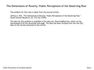
The Dimensions of Poverty: Public Perceptions of the Deserving Poor. The problem for this class is taken from the journal article: Jeffrey A. Will, "The Dimensions of Poverty: Public Perceptions of the Deserving Poor." Social Science Research , 22, 312-332 (1993).

E N D
The Dimensions of Poverty: Public Perceptions of the Deserving Poor The problem for this class is taken from the journal article: Jeffrey A. Will, "The Dimensions of Poverty: Public Perceptions of the Deserving Poor." Social Science Research, 22, 312-332 (1993). The data for this problem is available in the data set, DeservingPoor.Sav, which can be downloaded from the download web page. The data has been recoded from the raw GSS data to the format presented in the article. Public Perceptions of the Deserving Poor
Stage 1 Summary: Definition Of The Research Problem Relationship to be Analyzed "Of particular interest will be an examination of those characteristics of poor families which are perceived by the public as indicators of the deservedness of persons to receive public assistance." (Page 317) Specifying the Dependent and Independent Variables The dependent variable is the weekly income that the respondent felt the vignette family deserved: AMT 'Total Amount Family Gets'. The independent variables are the randomly assigned characteristics of the vignette family: Public Perceptions of the Deserving Poor
Stage 1 Summary: Definition Of The Research Problem Method for including independent variables: standard, hierarchical, stepwise The question suggests the use of either standard multiple regression or stepwise regression to determine which characteristics have a significant relationship to the dependent variable. We will use standard multiple regression to maintain consistency with the article. Public Perceptions of the Deserving Poor
Stage 2 Summary: Develop The Analysis Plan: Sample Size Issues Missing data analysis There is no missing data in this analysis. Power to Detect Relationships: Page 165 of Text With over 9,000 cases, we exceed the dimensions of the power table, so R² values of less than 2% will be found to be statistically significant. Minimum Sample Size Requirement: 15-20 Cases Per Independent Variable We have 9,555 observations and 23 independent variables (including dummy-coded variables), for a ratio of 415 cases per independent variable. Public Perceptions of the Deserving Poor
Stage 2 Summary: Develop The Analysis Plan: Measurement Issues Incorporating Nonmetric Data with Dummy Variables All variables requiring dummy coding were recoded when the data set was constructed. Representing Curvilinear Effects with Polynomials We do not have any evidence of curvilinear effects at this point in the analysis. Representing Interaction or Moderator Effects We do not have any evidence at this point in the analysis that we should add interaction or moderator variables. Public Perceptions of the Deserving Poor
Stage 3 Summary: Evaluate Underlying Assumptions Metric Dependent Variable and Metric or Dummy-coded Independent Variables All of the variables in the analysis are metric or dummy-coded. Note that Family Savings was dichotomously coded as either 0 or 1000. This scheme will make the slope more interpretable. The omitted categories for each dummy-coded, nonmetric variable can be derived from Table 1 on page 320 which lists the original categories for each variable. Public Perceptions of the Deserving Poor
Stage 3 Summary: Evaluate Underlying Assumptions Normality of metric variables Because of the factorial design of the study where the independent variable conditions are randomly assigned to respondents, we would not expect the metric independent variables to be normally distributed. Their distribution would reflect the number of times each condition was presented to a respondent. To the degree that the assignment was random, we would expect these variables to show a uniform distribution, i.e. be presented to the same number of respondents. This expectation is verified by the histograms of the variables: Age of Youngest Child, Number of Children in the Family, Child's Mother's Education, and Family Income. We would expect the dependent variable: Total Amount the Family Gets, which was a function of respondent feedback, to be more normally distributed. Though it fails the KS-Lilliefors, the histogram does indicate a pattern that can be described as approximating normality. Public Perceptions of the Deserving Poor
Stage 3 Summary: Evaluate Underlying Assumptions Linearity between metric independent variables and dependent variable The plots do not show any pattern of nonlinearity. (Note that these plots take a long time to run because of the large sample size.) Constant variance across categories of nonmetric independent variables The Levene test fails for the following: Mother Divorced, Father Unemployed and Not Looking, Mother Working Part-time, Mother Looking for Work, Mother Unemployed and Not Looking Because Only Minimum Wage Jobs Available. The only remedy for this problem would be a transformation of the dependent variable, but given the histogram of the dependent variable compared to the histograms of the transformations of the dependent variable, I will forego any transformations. Public Perceptions of the Deserving Poor
Stage 4: Compute the Statistics And Test Model Fit: Computations In this stage, we compute the actual statistics to be used in the analysis. Regression requires that we specify a variable selection method. The article uses a standard multiple regression. Compute the Regression Model The first task in this stage is to request the initial regression model and all of the statistical output we require for the analysis. Public Perceptions of the Deserving Poor
Request the Regression Analysis Public Perceptions of the Deserving Poor
Specify the Dependent and Independent Variables Public Perceptions of the Deserving Poor
Specify the Statistics Options Public Perceptions of the Deserving Poor
Specify the Plots to Include in the Output Public Perceptions of the Deserving Poor
Specify Diagnostic Statistics to Save to the Data Set Public Perceptions of the Deserving Poor
Complete the Regression Analysis Request Public Perceptions of the Deserving Poor
Stage 4: Compute the Statistics And Test Model Fit: Model Fit In this stage, we examine the relationships between our independent variables and the dependent variable. First, we look at the test of R Square which represents the relationship between the dependent variable and the set of independent variables. This analysis tests the hypothesis that there is no relationship between the dependent variable and the set of independent variables, i.e. the null hypothesis is: R² = 0. If we cannot reject this null hypothesis, then our analysis is concluded; there is no relationship between the dependent variable and the independent variables that we can interpret. If we reject the null hypothesis and conclude that there is a relationship between the dependent variable and the set of independent variables, then we examine the table of coefficients to identify which independent variables have a statistically significant individual relationship with the dependent variable. For each independent variable in the analysis, a t-test is computed that the slope of the regression line (B) between the independent variable and the dependent variable is not zero. The null hypothesis is that the slope is zero, i.e. B = 0, implying that the independent variable has no impact or relationship on scores on the dependent variable. Public Perceptions of the Deserving Poor
Significance Test of the Coefficient of Determination: R Square The R² of .145 is statistically significant with a probability for the F-test less than 0.0001. The author notes in a footnote on page 327 that the size of R² which he obtains is typical for this type of study. Public Perceptions of the Deserving Poor
Significance Test of Individual Regression Coefficients The individual variables that had a statistically significant relationship to the dependent variable are highlighted in the table on the next slide, using a significance level of 0.01 because the sample size was so large. With the exception of child's mother's education (highlighted in green), our findings concur with the author’s discussion on page 325-327. We find a statistically significant inverse relationship between mother's education and size of the award, while the author's coefficient is positive and statistically significant. I cannot explain this discrepancy. Usually, a difference in sign indicates a reversal in the coding scheme, but I think I used the same scheme described by the author. The difference is not inconsequential; in my analysis, respondents were less generous with mothers who had more education, while in the author's analysis, respondents were more generous to mothers with greater education. We obtain coefficients that differ slightly from the author due to unreconciled differences in the subjects included in the study, i.e. I had 9,555 observations, while he had 9,537 observations in his analysis. Public Perceptions of the Deserving Poor
Significance Test of Individual Regression Coefficients Public Perceptions of the Deserving Poor
Stage 4: Compute the Statistics And Test Model Fit Meeting Assumptions Using output from the regression analysis to examine the conformity of the regression analysis to the regression assumptions is often referred to as "Residual Analysis" because if focuses on the component of the variance which our regression model cannot explain. Using the regression equation, we can estimate the value of the dependent variable for each case in our sample. This estimate will differ from the actual score for each case by an amount referred to as the residual. Residuals are a measure of unexplained variance or error that remains in the dependent variable that cannot be explained or predicted by the regression equation. Public Perceptions of the Deserving Poor
Linearity and Constant Variance for the Dependent Variable: Residual Plot The residual plot shows the pattern that is associated with a discrete dependent variable. There is no evidence of nonlinearity. In the plot of residuals, we see that the spread of the residuals is constant (same height) across of the values for the dependent variable, so we do not have a pattern of heteroscedasticity. Public Perceptions of the Deserving Poor
Normal Distribution of Residuals: Normality Plot of Residuals If we examine the normal p-p plot produced by the regression, the residuals appear to be normally distributed. Public Perceptions of the Deserving Poor
Linearity of Independent Variables: Partial Plots The partial plots, such as the one for Family Income, do not suggest a pattern of nonlinearity. Public Perceptions of the Deserving Poor
Independence of Residuals: Durbin-Watson Statistic We obtain a value of 1.034 for the Durbin-Watson test, suggesting that there is a pattern of serial correlation within the data set. With the number of variables and cases in our analysis, the critical values for the probability table are 1.57 for the lower tail and 1.78 for the upper tail. Since our value of 1.03 falls outside this range, we reject the null hypothesis that serial correlation is zero, and conclude that serial correlation is a problem in this analysis. However, this evidence of serial correlation is an artifact of the way the data set was structured, i.e. each respondent reviewed seven vignettes, which were added to the data set in sequential order. There is a tendency for a respondent to be generous or punitive across cases he or she reviewed, as shown in the casewise table on the next slide (which I computed by running the regression again requesting that the casewise plot contain all cases instead of those with standardized residuals greater than 3.0). Public Perceptions of the Deserving Poor
Independence of Residuals: Durbin-Watson Statistic From this table, we can see that the same respondent who reviewed cases 8 through 14 said that the families should receive $200-$300 per month. The respondent who reviewed cases 22 through 28 was more generous, suggesting benefits of $400-$500 per month. The standardized residuals for the first individual have small negative values, while the standardized residuals for the second individual were high positive residuals. Since the variable that indicates the identify of the respondent (ID) is not included in the analysis, we can make this serial correlation problem disappear by sorting the cases in a different order. For example, I sorted the data set on the ‘randnum’ variable I created to produce the selection variable, ran the regression again, and found that the Durbin-Watson statistic had a value of 1.959, very close to the desired value of 2.0. Had the variable that produced the serial correlation been required for the analysis, e.g. a measure of time, re-sorting the data set would not remove the problem, and we would have to look at other strategies for correcting for this problem. Public Perceptions of the Deserving Poor
Identifying Dependent Variable Outliers:Casewise Plot of Standardized Residuals While it would appear that we have a large number of residuals larger than 3.0, we should remember that our sample is over 9,000 cases and the proportion of residuals is not excessive for that size sample (0.1% of all cases are outliers). Public Perceptions of the Deserving Poor
Identifying Influential Cases: Cook's Distance • Cook's distance identifies cases that are influential or have a large effect on the regression solution and may be distorting the solution for the remaining cases in the analysis. While we cannot associate a probability with Cook's distance, we can identify problematic cases that have a score larger than the criteria computed using the formula: 4/(n - k - 1), where n is the number of cases in the analysis and k is the number of independent variables. For this problem which has 9555 subjects who had nonmissing data and 23 independent variables, the formula equate to: 4 / (9555 - 23 - 1) = 0.00042. • A total of 566 cases had a Cook's distance of 0.00042 or larger, or about 6% of the sample. Since only 1 percent of the cases were outliers on the dependent variable, it is likely that the majority of these cases are outliers on the combination of independent variables. If that is the case, it could be argued that we should not consider omitting these cases because they are a consequence of the factorial design which randomly assigned the values or conditions to the independent variables. • If we rejected that argument and ran the regression without these cases, the results are even more positive. The R² value increases from 14.5% to 25.8%. Moreover, the number of variables with a significant individual relationship to the dependent variable increased, add the variables: • DADNOTLO 'Father Unemployed, Not Looking' • DADPRISO 'Father In Prison' • MOMNOTLO 'Mother Unemployed, Not Looking' • Though it is obvious that the influential cases have a negative impact on the analysis, we will retain these cases to maintain consistency with the author. Public Perceptions of the Deserving Poor
Stage 5: Interpret The Findings - Regression Coefficients Direction of relationship and contribution to dependent variable This is an instance where the unstandardized coefficients have a useful meaning in terms of the number of dollars associated with each characteristic of the welfare family, i.e. in terms of an allowance for need or a penalty. For example, if the father in the vignette was disabled, respondents tended to award $26 more per month to the family. If the father was unemployed and not looking for work, respondents reduced the award by $7 per month. Importance of Predictors The largest beta coefficients were associated with family income and number of children in the family, which logically are very important for estimation of needed welfare benefits. Impact of multicollinearity Multicollinearity does not appear to be a problem in this analysis. SPSS did not alert us to any tolerance problems. The correlations among independent variables were weak or very weak, a consequence of the factorial design of the study. Public Perceptions of the Deserving Poor
Stage 6: Validate The Model Interpreting adjusted R square Adjusted R Square (.143) is not much smaller than R Square (.145) indicating that over-fitting is not an issue for this problem. With over 9,000 cases in the study, it would be very unlikely that we would have too many independent variables in the analysis. Split-Sample Validation
Stage 6: Validate The Model The validation analysis suggests that the weak (almost moderate) relationship between family characteristics and amount of welfare seen as needed is generalizable to the larger population. There are five stable predictors: Number of children in family, Father disabled, Father unemployed and looking for work, Mother unemployed because only minimum wage jobs are available, and Family Income. Several other independent variables showed some pattern of relationship, but it was less consistent than these five predictors. The values of R and R² are consistent across analysis, suggesting that our findings are generalizable.