Software Reliability
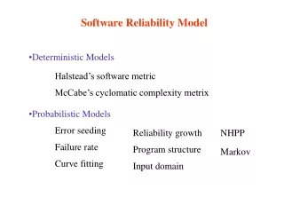
Software Reliability. ECE-355 Tutorial Jie Lian. Outline. Part I: Software Reliability Model Musa’s Basic Model Musa/Okumoto Logarithmic Model Part II: Control Flow Graph. Definition of Software Reliability.

Software Reliability
E N D
Presentation Transcript
Software Reliability ECE-355 TutorialJie Lian Software Reliability
Outline • Part I: Software Reliability Model • Musa’s Basic Model • Musa/Okumoto Logarithmic Model • Part II: Control Flow Graph Software Reliability
Definition of Software Reliability • Reliability is usually defined in terms of a statistical measure for the operation of a software system without a failure occurring • Software reliability is a measure for the probability of a software failure occurring • Two terms related to software reliability • Fault: a defect in the software, e.g. a bug in the code which may cause a failure • Failure: a derivation of the programs observed behavior from the required behavior Software Reliability
Parameters of Software Reliability • Average total number of failures (t) Average refers to n independent instantiations of an identical software. • Failure intensity (t) Number of failures per time unit, derivative of (t). • Mean Time To Failure (MTTF): • t may denote elapsed execution calendar or machine clock time Software Reliability
Importance of Software Reliability • In safety-critical systems, certain failures are fatal. This requires pushing reliability to very high levels at very high costs (code redundancy, hardware redundancy, recovery blocks, n version programming…). • In non-safety-critical systems a certain failure rate is usually tolerable. • This is a question of quality of service. • Which failure rate is tolerable is mainly a question of customer acceptance. (customer lifts receiver and receives neither fast busy nor dial tone one every 10/10000 calls?) • We will only talk about non-safety-critical systems Software Reliability
Software Reliability Growth Model (SRG) • Purpose of SRG models SRGs rely on observation of failure occurrence and try to predict future failure behavior • Two different SRG models (appr 40 models totally): • Musa linear model • Musa/Okomoto logarithmic model Software Reliability
Basic Assumptions of Musa’s Model • Faults are independent and distributed with constant rate of encounter. • Well mixed types of instructions, execution time between failures is large compared to instruction execution time. • Test space covers use space. (Tests selected from a complete set of use input sets). • Set of inputs for each run selected randomly. • All failures are observed, implied by definition. • Fault causing failure is corrected immediately, otherwise reoccurrence of that failure is not counted. Software Reliability
Musa’s Basic Model • Assumption: decrement in failure intensity function is constant. • Consequence: failure intensity is function of average number of failures experienced at any given point in time (= failure probability). • (): failure intensity. • 0: initial failure intensity at start of execution. • : average total number of failures at a given point in time. • v0: total number of failures over infinite time. Software Reliability
Example 1 • Assume that we are at some point of time t time units in the life cycle of a software system after it has been deployed. • Assume the program will experience 100 failures over infinite execution time. During the last t time unit interval 50 failures have been observed (and counted). The initially failure intensity was 10 failures per CPU hour. • Compute the current (at t) failure intensity: Software Reliability
Musa/Okumoto Logarithmic Model • Decrement per encountered failure decreases: : failure intensity decay parameter. • Example 2 • 0 = 10 failures per CPU hour. • =0.02/failure. • 50 failures have been experienced ( = 50). • Current failure intensity: Software Reliability
Model Extension (1) • Average total number of counted experienced failures () as a function of the elapsed execution time (). • For basic model • For logarithmic model Software Reliability
Example 3 (Basic Model) • 0 = 10 [failures/CPU hour]. • v0 = 100 (number of failures over infinite execution time). • = 10 CPU hours: • = 100 CPU hours: Software Reliability
Example 4 (Logarithmic Model) • 0 = 10 [failures/CPU hour]. • = 0.02 / failure. • = 10 CPU hours: • = 100 CPU hours: (63 in basic model) (100 in basic model) Software Reliability
Model Extension (2) • Failure intensity as a function of execution time. • For basic model: • For logarithmic Poisson model Software Reliability
Example 5 (Basic Model) • 0 = 10 [failures/CPU hour]. • v0 = 100 (number of failures over infinite execution time). • = 10 CPU hours: • = 100 CPU hours: Software Reliability
Example 6 (Logarithmic Model) • 0 = 10 [failures/CPU hour]. = 0.02 / failure. • = 10 CPU hours: • = 100 CPU hours: (3.68 in basic model) (0.000454 in basic model) Software Reliability
Model Discussion • Comparison of basic and logarithmic model: • Basic model assumes that there is a 0 failure intensity, logarithmic model assumes convergence to 0 failure intensity. • Basic model assumes a finite number of failures in the system, logarithmic model assumes infinite number. • Parameter estimation is major problem: 0, , and v0. Usually obtained from: • system test, • observation of operational system, • by comparison with values from similar projects. Software Reliability
Part II: Control Flow Graph (CFG) • A graph representation of a set of statements is called a flow graph or control flow graph. • Nodes in the flow graph represent computations and the edges represent the flow of control. • A basic block is a sequence of consecutive three-address statements in which flow of control enters at the beginning and leaves at the end without halt or possibility of branching except at the end. • A CFG consists of a set of basic blocks. Software Reliability
Three-Address Statements • Assignment statements of the form x: = yopz or x: = opz, where op is a binary or unary arithmetic or logical operation. • Copy statements x: = y where the value of y is assigned to x. • Unconditional jump goto L. Execution jumps to the statement labeled by L. • Conditional jump if x relop y goto L. • Indexed assignments of the form x: = y[i] and x[i] := y. • Address and pointer assignments of the form x := &y, x := *y, and *x := y. • Param x and call p, n, and return y, where return value of y is optional. For a procedure call p(x1, x2, … , xn), the transformed three-address statements are: param x1 param x2 … param xn, call p, n Software Reliability
Partition into Basic Blocks • Input: A sequence of three-address statements. • Output: A list of basic blocks with each three-address statements in exactly one block. • Method • Determining leaders (the first statement of basic blocks) by three rules: • The first statement is a leader. • Any statement that is the target of a conditional or unconditional goto is a leader. • Any statement that immediately follows a goto or conditional goto statement is a leader. • For each leader, its basic block consists of the leader and all statements up to but not including the next leader or the end of the program. Software Reliability
Example • … • 1 I = 1; • TI = TV = 0; • sum = 0; • 2 IF (v[I] == –999) GOTO 10 • 3 IF (TI >= 1) GOTO 10 • 4 TI++; • 5 IF (v[I] < min) GOTO 8 • 6 IF (v[I] > max) GOTO 8 • 7 TV++; • sum = sum + v[I]; • 8 I++; • 9 GOTO 2 • 10 IF (TV <= 0) GOTO 12 • av = sum/TV; • goto 13 • av = –999; • … I = 1; TI = TV = 0; sum = 0;DO WHILE (v[I] <> –999 and TI < 1) { TI++; IF (v[I] >= min and v[I] <= max) { TV++; sum = sum + v[I]; } I++; } IF TV >0 ) av = sum/TV; ELSE av = –999 ; Basic Block While loop IF ELSE We do not strictly follow the transformation from source code to three-address statements. Note that each statement with a label is a leader. Software Reliability
Transformation from Basic Blocks to CFG • … • 1 I = 1; • TI = TV = 0; • sum = 0; • 2 IF (v[I] == –999) GOTO 10 • 3 IF (TI >= 1) GOTO 10 • 4 TI++; • 5 IF (v[I] < min) GOTO 8 • 6 IF (v[I] > max) GOTO 8 • 7 TV++; • sum = sum + v[I]; • 8 I++; • 9 GOTO 2 • 10 IF (TV <= 0) GOTO 12 • av = sum/TV; • goto 13 • av = –999; • … 1 predicate node 2 3 R1 4 R4 10 5 R2 6 R5 11 12 R3 8 7 13 9 R6 Outer region Software Reliability
Cyclomatic Complexity • McCabe’s cyclomatic complexity • V(G) = E – N + 2, E: number of edges, N: number of nodes. • V(G) = p + 1, p is a number of predicate (decision) nodes. • V(G) = number of regions (area surrounded by nodes/edges). • V(G): upper bound on the number of independent paths • Independent path: A path with at least one new node/edge. • Example (pp. 22) : • V(G) = E – N + 2 = 17 – 13 + 2 = 6 • V(G) = p + 1 = 5 + 1 = 6 • V(G) = 6 • Advantage: # of test cases is proportional to the program size. Software Reliability
References [1] Musa, JD, Iannino, A. and Okumoto, K., “Software Reliability: Measurement, Prediction, Application”, McGraw-Hill Book Company, NY, 1987. [2] A. V. Aho, R. Sethi, and J. Ullman, "Compilers: Principles, Techniques, and Tools", Addison-Wesley, Reading, MA, 1986. Software Reliability