Download
1 / 54
560 likes | 691 Vues
This document defines key software metrics, including measures, metrics, and indicators, highlighting their importance in software development and maintenance. It discusses the objectives of measurement—understanding processes, controlling projects, and improving products. We cover process metrics focusing on quality, project metrics for assessing schedule and quality, and product metrics analyzing complexity and effectiveness. Key principles for effective measurement include clear objectives, automation of collection and analysis, and the establishment of interpretative guidelines. Learn how to implement these metrics to enhance software quality.

E N D
Definition • Measure: A quantitative indication of the extent, amount, dimensions, capacity, or size of some attribute of a product or process. • Metric: A quantitative measure of the degree to which a system, component, or process possesses a given attribute. A comparison of 2 or more measures. • Indicator:A metric or combination of metrics that provide insight into the software process, a software project or the product.
Why Do We Measure? • To understand what is happening during development and maintenance. • To control what is happening on our projects. • To improve our process and products.
A Good Manager Measures process process metrics project metrics measurement product metrics product What do we use as a basis? •size? •function?
Process Metrics • majority focus on quality achieved as a consequence of a repeatable or managed process • statistical SQA data • error categorization & analysis • defect removal efficiency • propagation from phase to phase
DRE = (errors) / (errors + defects) where errors = problems found before release defects = problems found after release Defect Removal Efficiency
Project Metrics • Objectives: • To minimize the development schedule • To assess product quality on an ongoing basis. • Examples: • Effort/time per SE task • Errors uncovered per review hour • Scheduled vs. actual milestone dates • Changes (number) and their characteristics • Distribution of effort on SE tasks
Product Metrics • Objectives: • focus on the quality of deliverables • Examples: • measures of analysis model • complexity of the design • internal algorithmic complexity • architectural complexity • data flow complexity • code measures (e.g., Halstead) • measures of process effectiveness • e.g., defect removal efficiency
Measurement Process • Formulation • Collection • Analysis • Interpretation • Feedback
Formulation Principles • The objectives of measurement should be established before data collection begins • Each technical metric should be defined in an unambiguous manner. • Metrics should be derived based on a theory that is valid for the domain of application. • Metrics should be tailored to best accommodate specific products and processes.
Collection & Analysis Principles • Whenever possible, data collection and analysis should be automated. • Valid statistical techniques should be applied to establish relationships between internal product attributes and external quality characteristics. • Interpretative guidelines and recommendations should be established for each metric.
Attributes Of Effective Software Metrics • Simple and Computable • Empirically and Intuitively • Consistent and Objective • Programming language independent • An effective mechanism for quality feedback
Product Operation Correctness Reliability Usability Integrity Efficiency Product Revision Maintainability Testability Flexibility Product Transition Reusability Portability Interoperability Measuring Software Quality: McCall’s Quality Factors
Reliability Consistency Accuracy Error-tolerance Simplicity Maintainability Concision Consistency Modularity Self-documentation simplicity Measuring Software Quality: McCall’s Quality Factors
Unambiguous Complete Correct Understandable Verifiable Internally consistent Externally consistent Achievable Concise Design independent Traceable Modifiable Electronically stored Executable/Interpretable Annotated by relative importance Annotated by relative stability Annotated by version Not redundant At right level of detail Precise Reusable Traced Organized Cross-referenced Measuring Quality in Software Requirements Specification (SRS)
Metrics for SRS Attributes • nf = functional requirements • nnf = non-functional requirements • nr = total requirements = nf + nnf
Unambiguous • A SRS is unambiguous if and only if every requirement stated therein has only one possible interpretation. • Metric: nui is the number of requirements for which all reviewers presented identical interpretations. 0 - every requirement has multiple interpretation 1 - every requirement has a unique interpretation
Completeness • A SRS is complete if everything that the software is supposed to do is included in the SRS. • Metric: • nA is the number of requirements in block A
Correctness • A SRS is correct if and only if every requirement represents something required of the system to be built • Metric: • nC is the number of correct requirements • nI is the number of incorrect requirements
Understandable • A SRS is understandable if all classes of SRS readers can easily comprehend the meaning of all requirements with a minimum of explanation. • Metric: nur is the number of requirements for which all reviewers thought they understood.
Concise • A SRS is concise if it is as short as possible without adversely affecting any other quality of the SRS. • Metric: • size is the number of pages
Not Redundant • A SRS is redundant if the same requirement is stated more than one. • Metric: • nf is the actual functions specified • nu is the actual unique functions specified
High-level Design Metrics • High-level design metrics focus on characteristics of the program architecture with an emphasis on the architectural structural and the effectiveness of modules • Metrics: • Card and Glass (1990) • Henry and Kafura (1981) • Fenton (1991)
Card And Glass (1990) • 3 software design complexity measures: • structural complexity • data complexity • system complexity
Card And Glass (1990) • Structural complexity (S(i)) where fout is the fan-out of module i • Data complexity (D(i)) where v(i) is the number of input and output variables that are passed to and from module i • System complexity (C(i))
Henry & Kafura (1981) where length (i) = the number of programming language statements in module i fin(i) = the number of fan-in of module i fout(i) = the number of fan-out of module i • fan-in = the number of local flows of information that terminate at a module + the number of data structures from which information is retrieved. • Fan-out = the number of local flows of information that emanate from a module plus_the number of data structures that are updated by that module
WC doc wc doc wc FD CW DR name doc doc err name doc, cw doc doc GDN RD FWS PW doc DOC
Fenton (1991) • Measure of the connectivity density of the architecture and a simple indication of the coupling of the architecture. r = a/n r = arc-to-node ratio a = the number of arcs (lines of control) n = the number of nodes (modules) • Depth = the longest path from the root (top) to a leaf node • Width = maximum number of nodes at any one level of the architecture
Component-level Design Metrics • Cohesion Metrics • Bieman and Ott (1994) • Coupling Metrics • Dhama (1995) • Complexity Metrics • McCabe (1976)
Bieman and Ott (1994) • Data slice is a backward walk through a module that looks for data values that affect the module location at which the walk began. • Data token are variables and constants defined for a module. • Glue tokens are data tokens that lie on one or more data slice. • Superglue tokens are the data tokens that are common to every data slice in a module.
Bieman and Ott (1994) • Strong functional cohesion (SFC) SFC(i) = SG(SA(i))/tokens (i) SG(SA(i)) = superglue tokens
Procedure Sum and Product (N : Integer; Var SumN, ProdN : Integer); Var I : Integer Begin SumN : = 0; ProdN : = 1; For I : = 1 to N do begin SumN : = SumN + I ProdN: = ProdN + I End; End;
Data Slide for SumN ( N : Integer; Var SumN, ProdN : Integer); Var I : Integer Begin SumN : = 0; ProdN : = 1; For I : = 1 to N do begin SumN : = SumN + I ProdN: = ProdN + I End; End; Data Slice for SumN = N1·SumN1·I1·SumN2·01·I2·12·N2·SumN3·SumN4·I3
Data Slide for ProdN ( N : Integer; Var SumN, ProdN : Integer); Var I : Integer Begin SumN : = 0; ProdN : = 1; For I : = 1 to N do begin SumN : = SumN + I ProdN: = ProdN + I End; End; Data Slice for ProdN = N1·ProdN1·I1·ProdN2·11·I2·12·N2·ProdN3·ProdN4·I4
Super Glue S1 S2 S3 I I I Super Glue I I I I I I Super Glue I I I Glue I I Glue
Functional Cohesion • Strong functional cohesion (SFC) SFC(i) = SG(SA(i))/tokens (i) SG(SA(i)) = superglue tokens SG(SumAndProduct)= 5/17= 0.204
Dhama (1995) • Data and control flow coupling • di = number of input data parameters • ci = number of input control parameters • do = number of output data parameters • co = number of output control parameters • Global coupling • gd = number of global variables used as data • gc = number of global variables used as control • Environmental coupling • w = number of modules called (fan-out) • r = number of modules calling the module under consideration (fan-in)
Dhama (1995) • Coupling metric (mc) mc = k/M, where k = 1 M = di + a* ci + do + b* co + c* gc + w + r where a=b=c=2
Coupling Metric - Example MODULE 1 Package sort1 is type array_type is arrary (1..1000) of integer; procedure sort1 (n: in integer; to_be_sorted: in out array_type; a_or_d: in character) is location, temp: integer; begin for start in 1..n loop location := start; loop to get min or max each time for i in (start + 1)..n loop if a_or_d = ‘d’ then if to_be_sorted(i) > to_be_sorted(location) then location := i; endif; else if to_be_sorted(i) < to_be_sorted(location) then location := i; endif endloop; temp := to_be_sorted(start); to_be_sorted(start) := to_be_sorted(location); to_be_sorted(location) := temp; endloop endsort1; endsort1;
Coupling Metric - Example MODULE2 Package sort2 is type array_type is arrary (1..1000) of integer; Procedure sort2 (n: in integer; to_be_sorted: in out array_type; a_or_d: in character); procedure find_max (n: in integer; to_be_sorted: in out array_type; location: in out integer); procedure find_min (n, start: in integer; to_be_sorted: in out array_type; location: in out integer); procedure exchange (start: in integer; to_be_sorted: in out array_type; location: in out integer); endsort2;
procedure find_max (n, start : in integer; to_be_sorted: in out array_type; location: in out integer); is begin location := start; for i in start + 1..n loop if to_be_sorted(i) > to_be_sorted(location) then location := i; endif; endloop end find_max; procedure find_min (n, start: in integer; to_be_sorted: in out array_type; location: in out integer) is begin location := start; for i in start + 1..n loop if to_be_sorted(i) < to_be_sorted(location) then location := i; endif; endloop end find_min; Coupling Metric - Example
procedure exchange (start: in integer; to_be_sorted: in out array_type; location: in out integer) is temp: integer; begin temp := to_be_sorted(start); to_be_sorted(start) := to_be_sorted(location); to_be_sorted(location) := temp; end exchange; Procedure sort2 (n: in integer; to_be_sorted: in out array_type; a_or_d: in character)is location : integer; begin for start in 1..n loop if a_or_d = ‘d’ then find_max(n, start, to_be_sorted, location); else find_min(n, start, to_be_sorted, location); endif; exchange(start, to_be_sorted, location); endloop; end sort2; end sort2; Coupling Metric - Example
McCabe (1976) • Cyclomatic Complexity (V(G)) • V(G) = the number of region of the flow graph + the area outside the graph • V(G) = E - N + 2 where E = the number of flow graph edges N = the number of flow graph nodes • V(G) = P + 1 where P = the number of predicate nodes
CASE IF Sequence Until Flow Graph Notation While
Node Edge 1 1 2,3 2 R2 6 4, 5 3 R3 7 8 R1 6 4 10 9 Region 7 8 5 R4 9 10 11 11 Cyclomatic Complexity - Example
Metrics for Testing • Size of the software • High-level design metric • Cyclomatic complexity
Metrics for Maintenance • Fix Backlog and Backlog Management Index • Fix Response Time • Percent Delinquent Fixes • Fix Quality • Software Maturity Index (SMI)
Number of problems closed during the month X 100% BMI = Number of problem arrivals during the month Fix Backlog and Backlog Management Index • Fix backlog is a work load statement for software maintenance. • It is a simple count of reported problems that remain opened at the end of each month or each week. • Backlog management index (BMI)
Fix Response Time • Fix response time metric = Mean time of all problems from open to closed