SPSS Session 3: Finding Differences Between Groups
This session focuses on how to analyze differences between two or more groups using SPSS. Participants will review key concepts from previous lectures, including the theory of probability, hypotheses testing, and the relationship between variability and standard deviation. The session will cover how to perform t-tests and ANOVAs in SPSS and interpret the results. Through practical examples, attendees will learn to assess the significance of differences in mean scores, understand statistical outputs, and apply these techniques to real-world social work research scenarios.

SPSS Session 3: Finding Differences Between Groups
E N D
Presentation Transcript
Learning Objectives • Review Lectures from 8 and 9 • Understand how to test for differences between two or more groups • Describe the relationship between variability and standard deviation of means • Be able to conduct t-tests and ANOVAs within SPSS • From the statistical output, be able to discuss results of analyses using t-tests and ANOVAs
Review of Lecture 8 • Defined and discussed the theory and rules of probability • Calculated probability and created a probability distribution with example data • Described the characteristics of a normal curve and interpreted a normal curve using example data
Review from Lecture 9 • Defined research hypothesis, null hypothesis and statistically significance • Discussed the basic requirements for testing the difference between two means • Defined and described the difference between the alpha value and P value, and Type I and Type II errors • Calculated the difference between the means (t-ratio) using example data through advanced study
Testing for Differences between Groups • Often times in social work research, we wish to know if the differences between two groups is significant. • No two groups of people are alike, but are their dissimilarities important? • That is to say, are the differences significant or did these differences likely happen by chance? • Think about comparing p-value to α.
Testing for Differences between Groups • Testing for differences between groups of people on some score or measure is reliant on: • The average scores for each group on that measure (mean scores) • The variability of each group’s scores on that measure (standard deviation scores) • Mean and standard deviation scores are very important when comparing groups
Standard Deviation Scores • Standard Deviation (SD) is an important piece of statistical information • Stand Deviation scores indicate the extent to which the data cluster around the mean of a distribution. • It is the most common score of “data dispersion” and variability in a particular variable. • It is often reported in studies with the mean: • Example, “children in the study were 7.69 years of age on average (SD=4.85)”.
Deviation Scores • Deviation is the amount that an individual score is different from the mean score for that variable. • Recall that the children in the study were on average (mean) 7.69 years of age. • Deviation scores for specific cases then would be: • A child that is 10 years old would deviate from the mean by 2.31 years (10 - 7.69 =2.31) • A child that is 3 years old would deviate from the mean by -4.69 years (3 - 7.69 = -4.69)
Standard Deviation Scores • Standard Deviation scores (SD) are the square root of sum of all squared deviation scores for all individuals and divided by the total number of individuals minus one.
Standard Deviation Scores and Variability • Standard Deviation Scores (SD) are important as they give information about how closely the values in a distribution cluster around the mean. • Essentially, this is how much scores in a variable actually vary! • The next three slides demonstrate the variability. • Watch for the Standard Deviation Scores and changes in the histograms.
Histogram with Large SD scores • Mean = 50 • SD = 30
Histogram with Medium SD scores • Mean = 50 • SD = 14
Histogram with SD scores of 0 • Mean = 50 • SD = 0 (no variability)
Group Differences in Child Protection • In our child protection study, we wanted to for differences between two groups of parents. • All parents completed the General Health Questionnaire, and were categorized as having clinically scores or not. • Clinically elevated scores are those where the parents likely are experiencing severe psychiatric stress.
Group Differences in Child Protection • We hypothesized that there would be significant differences between these two groups of parents on their mean scores on the Family Environment Scale (FES) and the Strengths and Difficulty Questionnaire (SDQ). • The FES concerns three aspects of their social environment in their home: Family Cohesion, Family Expressiveness, and Family Conflict. • The SDQ total score concerns the parents’ views of the behaviour and social problems experienced by their child.
Testing for Differences between Groups • In order to test for differences between two groups based on their mean scores on a measure, we use a statistical test called a t-test. • t-tests use one nominal independent variable (IV) and one interval/ratio dependent variable (DV) • In this case: • GHQ groups (IV): Clinically elevated scores and not clinically elevated groups (one variable with two groups) • FES and SDQ scores (DV): interval/ratio level variables
T-tests Hypotheses • We hypothesized (research hypothesis) that there would be significant differences between these two groups of parents on their mean scores on the Family Environment Scale (FES) and the Strengths and Difficulty Questionnaire (SDQ). • Parents reporting greater stress would also have higher FES and SDQ scores. • Our null hypothesis states that there are no significant differences between these two groups of parents based on their mean scores on the FES and SDQ measures. • We have the data, so time to test!
T-tests Analysis Demonstrated in SPSS • When conducting a t-test, use the “Analyze” menu and select “Compare Means”. • In this case, we select “Independent Samples t-test” as the parents either have clinically elevated GHQ scores or they do not.
Firstly, we identify our DV called here as our “Test Variable(s)”. • Find “SDQ_TotalDif” in the list on the left and select it for the “Test Variable(s)”.
Next, we identify our IV and the particular groups of interest. • Select “GHQ_Cutoff_4” from the list on the left and select this variable for the “Grouping Variable”. GHQ scores use a clinical cutoff score of 4 or more, hence the variable name.
Now that the IV variable is identified, we have to tell SPSS which two groups we are using in the analysis. • This variable is coded as the following: • 0 = "Subclinical score, 3 or less" • 1 = "Clinically elevated score, 4 or more" • Knowing the coding for each group, select “Define Groups…” • Specify the two groups as: • Group 1: 0 • Group 2: 1 • Click “Continue”
Identify the values for each group in the variable based on how the variable is coded. After clicking “Continue”, the “Grouping Variable” shows the grouping numbers. Now click “OK”.
T-tests Analysis Results in SPSS • Now we see the results of the test between the two parent groups on the SDQ measure. • The first table give the mean and standard deviations scores on the SDQ measure for group of parents with clinically elevated GHQ scores (42 people) and those without the elevated scores (53 people).
T-tests Analysis Results in SPSS • The mean SDQ scores for each group do not appear significantly different. • The group with the elevated GHQ scores had a mean SDQ score of 20.38 (SD=6.868). • The group of parents without an elevated GHQ score actually had lower mean SDQ scores of 20.94 (SD=7.202). • We had hypothesized that parents with elevated GHQ scores would also rate their children as having more total difficulties as rated by the SDQ (research hypothesis).
T-tests Analysis Results in SPSS • To see if these results likely occurred by chance, or if there is a statistically significant difference between these two groups of parents, we look to the next table for the results of the t-test.
From the table below, we see the t-test score of t=.386 and a p-value of .701 shown here as “Sig. (2-tailed)” with 93 degrees of freedom (“df”). • Because the p-value of .701 is greater than our α = .05 level of significance, we say that we failed to reject our null hypothesis. • These results likely happened by chance, and we cannot confirm our research hypothesis.
T-tests Analysis Results in SPSS • Our null hypothesis stated that there were no statistically significant differences between these two groups of parents based on their SDQ means scores. From our data, this appears to be the case. • SDQ scores were not significantly different (t=.386, df=93, p>.05) between parents with clinically elevated GHQ scores (mean SDQ scores of 20.38, SD=6.868) and those parents without clinically elevated GHQ scores (mean SDQ scores of 20.94, SD=7.202). • Parents with increased levels of stress did not rate their children has having greater behavioural and social problems when compared to the parents reporting lower levels of stress.
T-tests Analysis in SPSS: Second Example • For a second example, we wanted to know if these same two groups of parents differed in terms of their family environment. • We used the Conflict subscale of the Family Environment Scale as a measure of their family social environment. • Our research hypothesis is that the group of parents with clinically elevated GHQ scores would have significantly higher FES-Conflict scores when compared to the group of parents without clinically elevated scores. • Our null hypothesis stated that there is no difference between these groups of parents based on their FES-Conflict scores.
T-tests Analysis in SPSS: Second Example • To test this second research hypothesis, we again select the “Analyze” menu and select “Compare Means”. • Again, we use “Independent Samples t-test” to test for differences between to independent groups of parents.
T-tests Analysis in SPSS: Second Example • From the window for “Independent-Samples T Test”, the previous analysis is shown. • Because we are interested in testing the new DV of FES-Conflict scores, we remove “SDQ_TotalDif” from the list and replace it with “FES_Conflict” from the list on the right. • The “Grouping Variable” is still set from the previous analysis and does not need changing. • As the analysis is set, we click “OK” for the results.
T-tests Results in SPSS: Second Example • From the results in the output window, we see the first table with the mean and standard deviation scores for each group. • We see that the mean FES-Conflict scores for the clinically elevated group (mean=5.19, SD=2.32) appears to be higher than the group of parents without clinically elevated scores (mean=3.87, SD=2.72). • To find if this difference is statistically significant, we look to the next table in the output.
From the table below, we see the t-test score of t=-2.511 and a p-value of .014 shown here as “Sig. (2-tailed)” with 93 degrees of freedom (“df”). • Because the p-value of .014 is less than our α = .05 level of significance, we say that succeeded in rejecting our null hypothesis. • These results were unlikely to have happened by chance, and we accept our research hypothesis.
Our null hypothesis stated that there were no statistically significant differences between these two groups of parents based on their FES-Conflict means scores. From our data, this appears not to be the case. • FES-Conflictscores were significantly different (t=-2.511, df=93, p<.05) between parents with clinically elevated GHQ scores (mean FES-Conflictscores of 5.19, SD=2.32) and those parents without clinically elevated GHQ scores (mean FES-Conflictscores of 3.87, SD=2.72).
T-tests Results in SPSS: Second Example • From the results of this second t-test, we can conclude that parents with clinically elevated GHQ scores reported significantly greater amounts of social conflict in their family environments.
Analysis of Variance (ANOVA):Testing for Differences between Three or More Groups
Analysis of Variance (ANOVA) • Where T-tests look for differences between only two groups, Analysis of Variance (ANOVA) tests for similar differences between three or more groups. • The independent variable is a nominal or ordinal variable with three or more categories • The dependent variable is a interval/ratio variable
Analysis of Variance (ANOVA) • The null hypothesis for an ANOVA test is that the mean score for each group on a particular measure will not significant differ from any other group. • The research hypothesis is usually that some group will be significant different from another group. • The ANOVA test produces a statistical score called a “F-value” through a “F test”.
Analysis of Variance (ANOVA) • The logic behind the ANOVA test is that the differences within a group of people is less so than those differences between the three or more groups. • ANOVA tests become a comparison of between group differences and within group differences. • Hence, it is an ANALYSIS of VARIANCE between groups compared to VARIANCE within each group. • T-tests are actually a mathematically simplified version of an ANOVA because it only needs to compare two groups!
The Two Parts of ANOVA First Step Second Step If the F-test is significant (p<.05), it means that there is one group significantly different from another. The second part of an ANOVA is to which group(s) are different. This is called a “post hoc” test meaning “after that” Post Hoc tests can be conducted many different ways. • ANOVA tests are conducted in two parts. • The first step is to test whether any group is significantly different from any other group. • This first step uses a F-test and is called an “omnibus” test meaning an “over all” test.
ANOVA Examples in Child Protection • For our child protection study, we wanted to test for differences between three groups of parents based on two different measures. • Using the Previous Involvement variable, we have all of the cases categorized in one of the following ways: • Cases with a history of occasional child protection involvement • Cases with a long standing history of child protection involvement • Cases with no history of child protection involvement
ANOVA Examples in Child Protection • Based on these three groups of parents and cases, we wanted to test for differences between them on two measures: • Family Environment Scale – Family Cohesion • We would expect that families with long standing or occasional involvement would have less family cohesion than families with no prior involvement with child protection services. • General Health Questionnaire – Total Score • We would expect that families with long standing or occasional involvement would have higher levels of psychological distress compared to families with no prior involvement with child protection services. • The null hypothesis for each test is that there are no differences between the three groups of cases based on any measure or score.
ANOVA Example: 1. Family Cohesion • Testing for differences between these three groups of cases based on the FES – Cohesion scores. • We need to find “Compare Means” under the “Analyze” menu. • Under “Compare Means”, select “One-Way ANOVA”
ANOVA Example: 1. Family Cohesion • Once “One-Way ANOVA” is selected a new window for ANOVA will appear
ANOVA Example: 1. Family Cohesion • First, we need to add the Dependent Variable which is the FES – Cohesion scores to the “Dependent List”. • Find this variable on the list on the left and add it to this list.
ANOVA Example: 1. Family Cohesion • Now we need to add the Independent Variable to the “Factor” list. • The Independent Variable is the groups of cases called “Previous_Involvement”
ANOVA Example: 1. Family Cohesion • This ANOVA test will now search for differences between the three groups, but it will not yet test for where exactly the differences exist. • This is the “omnibus test” portion. • We need to ask the ANOVA test also to conduct the “post hoc” test to find which group or groups are significantly different from other groups. • We do this by selecting a post hoc test from the “Post Hoc” option on the right.