Application-Level Scheduling in Distributed Heterogeneous Networks
This document explores application-level scheduling on distributed heterogeneous networks, with a focus on programming paradigms and algorithms relevant to parallel computing. Topics include embarrassingly parallel programs, master/slave programs, Monte Carlo methods, and iterative stencil computations such as the Jacobi algorithm for solving linear equations. It discusses the use of efficient strategies for convergence in Jacobi iterations, matrix representation, and the significance of communication patterns in solving large-scale computational problems. The insights presented are crucial for optimizing scientific applications using parallel programming techniques.

Application-Level Scheduling in Distributed Heterogeneous Networks
E N D
Presentation Transcript
Programming Paradigms and Algorithms W+A 3.1, 3.2, p. 178, 5.1, 5.3.3, Chapter 6, 9.2.8, 10.4.1, Kumar 12.1.3 1. Berman, F., Wolski, R., Figueira, S., Schopf, J. and Shao, G., "Application-Level Scheduling on Distributed Heterogeneous Networks," Proceedings of Supercomputing '96 (http:apples.ucsd.edu) CSE 160/Berman
Common Parallel Programming Paradigms • Embarrassingly parallel programs • Workqueue • Master/Slave programs • Monte Carlo methods • Regular, Iterative (Stencil) Computations • Pipelined Computations • Synchronous Computations CSE 160/Berman
Regular, Iterative Stencil Applications • Many scientific applications have the format Loop until some condition is true Perform computation which involvescommunicating with N,E,W,S neighborsof a point (5 point stencil) [Convergence test?] CSE 160/Berman
Stencil Example: Jacobi2D • Jacobi algorithm, also known as the method of simultaneous corrections is an iterative method for approximating the solution to a system of linear equations. • Jacobi addresses the problem of solving n linear equations in n unknowns Ax=b where the ith equation is or alternatively • a’s and b’s are known, want to solve for x’s CSE 160/Berman
Jacobi 2D Strategy • Jacobi strategy iterates until the computation converges to an exact solution, i.e. each iteration we solve where the values from the (k-1)st iteration are used to compute the values for the kth iteration • For important classes of problems, Jacobi converges to a “good” solution after O(logN) iterations [Leighton] • typically, the solution is approximated to a desired error threshold CSE 160/Berman
Jacobi 2D • Equation is most efficient to solve when most a’s are 0 • When most a’s entries are non-zero, A is dense • When most a’s are 0, A is sparse • Sparse matrices are regularly found in many scientific applications. CSE 160/Berman
La Place’s Equation • Jacobi strategy can be used effectively to solve sparse linear equations. • One such equation is La Place’s equation: • f is solved over a 2D space having coordinates x and y • If the distance between points (D) is small enough, f can be approximated by • These equations reduce to CSE 160/Berman
(x,y+D) (x,y) (x-D,y) (x+D,y) (x,y-D) La Place’s Equation • Note the relationship between the parameters • This forms a 4 point stencil Any update will involve only local communication! CSE 160/Berman
Solving La Place using Jacobi strategy • Note that in La Place equation, we want to solve for all f(x,y) which has 2 parameters • In Jacobi, we want to solve for x_i which has only 1 index • How do we convert f(x,y) into x_i ? • Associate x_i’s with the f(x,y)’s by distributing them in the f 2D matrix in row-major (natural) order • For an nxn matrix, there are then nxnx_i’s, so the A matrix will need to be (nxn)X(nxn) CSE 160/Berman
Solving La Place using Jacobi strategy • When the x_i’s are distributed in the f 2D matrix in row-major (natural) order becomes CSE 160/Berman
Working backward • Now we want to work backward to find out what the A matrix and b vector will be for Jacobi • Our solution to the La Place equation gives us equations of this form • Rewriting, we get • So the b_i are 0, what is the A matrix? CSE 160/Berman
Finding the A matrix • Each row only at most 5 non-zero entries • All entries on the diagonal are 4 N=9, n=3: CSE 160/Berman
Jacobi Implementation Strategy • An initial guess is made for all the unknowns, typically x_i = b_i • New values for the x_i’s are calculated using the iteration equations • The updated values are substituted in the iteration equations and the process repeats again • The user provides a "termination condition" to end the iteration. • An example termination condition is errorthreshold. CSE 160/Berman
Data Parallel Jacobi 2D Pseudo-code [Initialize ghost regions] for (i=1; i<=N; i++) x[0][i] = north[i]; x[N+1][i] = south[i]; x[i][0] = west[i]; x[i][N+1] = east[i]; [Initialize matrix] for (i=1; i<=N; i++) for (j=1; j<=N; j++) x[i][j] = initvalue; [Iterative refinement of x until values converge] while (maxdiff > CONVERG) [Update x array] for (i=1; i<=N; i++) for (j=1; j<=N; j++) newx[i][j] = ¼ (x[i-1][j] + x[i][j+1] + x[i+1][j] + x[i][j-1]); [Convergence test] maxdiff = 0; for (i=1; i<=N; i++) for (j=1; j<=N; j++) maxdiff = max(maxdiff, |newx[i][j]-x[i][j]|); x[i][j] = newx[i][j]; CSE 160/Berman
Jacobi2D Programming Issues • Synchronization • Should we synchronize between iterations? Between multiple iterations? • Should we tag information and let the application run asynchronously? (How bad can things get?) • How often should we test for convergence? • How important is it to know when we’re done? • How expensive is it? CSE 160/Berman
Jacobi2D Programming Issues • Block decomposition or strip decomposition? • How big should the blocks or strips be? • How should blocks/strips be allocated to processors? Block Uniform Strip Non-uniform Strip CSE 160/Berman
HPF-Style Data Decompositions • 1D (Processors P0 P1 P2 P3 , tasks 0-15) • Block decomposition (Task i allocated to processor floor (i/p)) • Cyclic decomposition (Task i allocated to processor i mod p) • Block-Cycle Decomposition (Block i allocated to processor i mod p) Block Cyclic Block-cyclic CSE 160/Berman
HPF-Style Data Decompositions • 2D • Each dimension partitioned by block, cyclic, block-cyclic or * (do nothing) • Useful set of uniform decompositions can be constructed [Block, Block] [Block, *] [* , Cyclic] CSE 160/Berman
Jacobi on a Cluster • If each partition of Jacobi is executed on a processor in a lab cluster, we can no longer assume we have dedicated processors and network • In particular, the performance exhibited by the cluster will vary over time and with load • How can we go about developing a performance-efficient implementation in a more dynamic environment? CSE 160/Berman
Jacobi AppLeS • We developed an AppLeS application scheduler • AppLeS = Application-Level Scheduler • AppLeS is scheduling agent which integrates with application to form a “Grid-aware” adaptive self-scheduling application • Targeted Jacobi AppLeS to a distributed clustered environment CSE 160/Berman
Resource Discovery Resource Selection SchedulePlanningand PerformanceModeling DecisionModel Schedule Deployment How Does AppLeS Work? AppLeS + application = self-scheduling application accessible resources feasible resource sets Grid Infrastructure NWS evaluatedschedules Resources “best” schedule
Sensor Interface Reporting Interface Forecaster Model 1 Model 2 Model 3 Network Weather Service (Wolski, U. Tenn.) • The NWS provides dynamic resource information for AppLeS • NWS is stand-alone system • NWS • monitors current system state • provides best forecast of resource load from multiple models
Feasible resources determined according to application-specific “distance” metric Choose fastest machine aslocus Compute distance Dfrom locus based on unit-sized application-specific benchmark D[locus,X] = |comp[unit,locus]-comp[unit,X]| + comm[W,E columns] Resources sorted according to distance from locus, forming a desirability list Feasible resource sets formed from initial subsets of sorted desirability list Next step: plan a schedule for each feasible resource set Scheduler will choose schedule with best predicted execution time Jacobi2D AppLeS Resource Selector
Execution time for ith strip whereload= predicted percentage of CPU time available (NWS) comm = time to send and receive messages factored by predicted BW (NWS) AppLeS uses time-balancingto determine best partition on a given set of resources Solve for P1 P2 P3 Jacobi2D Performance Model and Schedule Planning
Jacobi2D Experiments • Experiments compare • Compile-time block [HPF] partitioning • Compile-time irregular strip partitioning [no NWS forecasts, no resource selection] • Run-time strip AppLeS partitioning • Runs for different partitioning methods performed back-to-back on production systems • Average execution time recorded • Distributed UCSD/SDSC platform: Sparcs, RS6000, Alpha Farm, SP-2
Representative Jacobi 2D AppLeS experiment Adaptive scheduling leverages deliverable performance of contended system Spike occurs when a gateway between PCL and SDSC goes down Subsequent AppLeS experiments avoid slow link Jacobi2D AppLeS Experiments