Logistic Regression

1. Logistic Regression

2. Outline • Review of simple and multiple regression • Simple Logistic Regression • The logistic function • Interpretation of coefficients • continuous predictor (X) • dichotomous categorical predictor (X) • categorical predictor with three or more levels (X) • Multiple Logistic Regression • Examples

3. Simple Linear Regression Model the mean of a numeric response Y as a function of a single predictor X, i.e. E(Y|X) = bo + b1f(x) Here f(x) is any function of X, e.g. f(x) = X E(Y|X) = bo + b1X (line) f(x) = ln(X)  E(Y|X) = bo + b1ln(X) (curved) The key is that E(Y|X) is a linear in theparameters bo and b1 but not necessarily in X.

4. =-value at x = 0 b1 w units b0 = Change in for every w units unit increase in x x 0 Simple Linear Regression ^ b0 = Estimated Intercept Interpretable only if x = 0 is a value of particular interest. ^ ^ ^ b1 = Estimated Slope = estimated change in the mean of Y for a unit change in X. Always interpretable!

5. Multiple Linear Regression We model the mean of a numeric response as linear combination of the predictors themselves or some functions based on the predictors, i.e. E(Y|X) = bo + b1X1+ b2X2 +…+ bpXp Here the terms in the model are the predictors E(Y|X) = bo + b1 f1(X)+b2 f2(X)+…+bk fk(X) Here the terms in the model are k different functions of the p predictors

6. Multiple Linear Regression For the classic multiple regression model E(Y|X) = bo + b1X1+ b2X2 +…+ bpXp the regression coefficients (bi) represent the estimated change in the mean of the response Y associated with a unit change in Xi while the other predictors are held constant. They measure the association between Y and Xiadjusted for the other predictors in the model.

7. General Linear Models • Family of regression models • Response Model Type • Continuous Linear regression • Counts Poisson regression • Survival times Cox model • Binomial Logistic regression • Uses • Control for potentially confounding factors • Model building , risk prediction

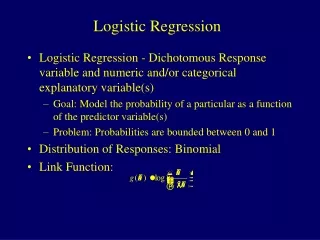
8. Logistic Regression • Models relationship betweenset of variables Xi • dichotomous (yes/no, smoker/nonsmoker,…) • categorical (social class, race, ...) • continuous (age, weight, gestational age, ...) and • dichotomous categorical response variable Y e.g. Success/Failure, Remission/No RemissionSurvived/Died, CHD/No CHD, Low Birth Weight/Normal Birth Weight, etc…

9. Logistic Regression Example: Coronary Heart Disease (CD) and AgeIn this study sampled individuals were examined for signs of CD (present = 1 / absent = 0) and the potential relationship between this outcome and their age (yrs.) was considered. … This is a portion of the raw data for the 100 subjects who participated in the study.

10. Logistic Regression • How can we analyze these data? Non-pooled t-test The mean age of the individuals with some signs of coronary heart disease is 51.28 years vs. 39.18 years for individuals without signs (t = 5.95, p < .0001).

11. Logistic Regression Simple Linear Regression? Smooth Regression Estimate? The smooth regression estimate is “S-shaped” but what does the estimated mean value represent? Answer: P(CD|Age)!!!!

12. Logistic Regression We can group individuals into age classes and look at the percentage/proportion showing signs of coronary heart disease. Notice the “S-shape” to the estimated proportions vs. age.

13. Logistic Function P(“Success”|X) X

14. Logit Transformation The logistic regression model is given by which is equivalent to This is called the Logit Transformation

15. Dichotomous Predictor Consider a dichotomous predictor (X) which represents the presence of risk (1 = present) Therefore the odds ratio (OR)

16. Dichotomous Predictor • Therefore, for the odds ratio associated with risk presence we have • Taking the natural logarithm we have thus the estimated regression coefficient associated with a 0-1 coded dichotomous predictor is the natural log of the OR associated with risk presence!!!

17. Logit is Directly Related to Odds The logistic model can be written This implies that the odds for success can be expressed as This relationship is the key to interpreting the coefficients in a logistic regression model !!

18. Dichotomous Predictor (+1/-1 coding) Consider a dichotomous predictor (X) which represents the presence of risk (1 = present) Therefore the odds ratio (OR)

19. Dichotomous Predictor • Therefore, for the odds ratio associated with risk presence we have • Taking the natural logarithm we have thus twice the estimated regression coefficient associated with a +1 / -1 coded dichotomous predictor is the natural log of the OR associated with risk presence!!!

20. Example: Age at 1st Pregnancy and Cervical Cancer Use Fit Model Y = Disease Status X = Risk Factor Status When the response Y is a dichotomous categorical variable the Personality box will automatically change to Nominal Logistic, i.e. Logistic Regression will be used. Remember when a dichotomous categorical predictor is used JMP uses +1/-1 coding. If you want you can code them as 0-1 and treat is as numeric.

21. Example: Age at 1st Pregnancy and Cervical Cancer Thus the estimated odds ratio is Women whose first pregnancy is at or before age 25 have 3.37 times the odds for developing cervical cancer than women whose 1st pregnancy occurs after age 25.

22. Example: Age at 1st Pregnancy and Cervical Cancer Thus the estimated odds ratio is Odds Ratio for disease associated with risk presence Risk Present

23. Example: Smoking and Low Birth Weight Use Fit Model Y = Low Birth Weight (Low, Norm) X = Smoking Status (Cig, NoCig) We estimate that women who smoker during pregnancy have 1.95 times higher odds for having a child with low birth weight than women who do not smoke cigarettes during pregnancy.

24. Example: Smoking and Low Birth Weight Find a 95% CI for OR 1st Find a 95% CI for b1 2nd Compute CI for OR = (e2LCL, e2UCL) (LCL,UCL) We estimate that the odds for having a low birth weight infant are between 1.86 and 2.05 times higher for smokers than non-smokers, with 95% confidence.

25. Example: Smoking and Low Birth Weight We might want to adjust for other potential confounding factors in our analysis of the risk associated with smoking during pregnancy. This is accomplished by simply adding these covariates to our model. Multiple Logistic Regression Model Before looking at some multiple logistic regression examples we need to look at how continuous predictors and categorical variables with 3 or levels are handled in these models and how associated OR’s are calculated.

26. Example 2: Signs of CD and Age Fit Model Y = CD (CD if signs present, No otherwise) X = Age (years) Consider the risk associated with a c year increase in age.

27. Example 2: Signs of CD and Age For example consider a 10 year increase in age, find the associated OR for showing signs of CD, i.e. c = 10 OR = ecb = e10*.111 = 3.03 Thus we estimate that the odds for exhibiting signs of CD increase threefold for each 10 years of age. Similar calculations could be done for other increments as well. For example for a c = 1 year increase OR = eb = e.111 = 1.18 or an 18% increase in odds per year

28. Example 2: Signs of CD and Age Can we assume that the increase in risk associated with a c unit increase is constant throughout one’s life? Is the increase going from 20  30 years of age the same as going from 50  60 years? If that assumption is not reasonable then one must be careful when discussing risk associated with a continuous predictor.

29. Example 3: Race and Low Birth Weight Calculate the odds for low birth weight for each race (Low, Norm) White Infants (reference group, missing in parameters) Black Infants Other Infants OR for Blacks vs. Whites= .167/.0805 = 2.075 OR for Others vs. Whites= .102/.0805 = 1.267 OR for Black vs. Others= .167/.102 = 1.637

30. Example 3: Race and Low Birth Weight Finding these directly using the estimated parameters is cumbersome. JMP will compute the Odds Ratio for each possible comparison and their reciprocals in case those are of interest as well. Odds Ratio column is odds for Low for Level 1 vs. Level 2. Reciprocal is odds for Low for Level 2 vs. Level 1. These are the easiest to interpret here as they represent increased risk.

31. Putting it all together Now that we have seen how to interpret each of the variable types in a logistic model we can consider multiple logistic regression models with all these variable types included in the model. We can then look at risk associated with certain factors adjusted for the other covariates included in the model.

32. Example 3: Smoking and Low Birth Weight • Consider again the risk associated with smoking but this time adjusting for the potential confounding effects of education level and age of the mother & father, race of the child, total number of prior pregnancies, number children born alive that are now dead, and gestational age of the infant. Several terms are not statistically significant and could consider using backwards elimination to simplify the model.

33. Example 3: Race and Low Birth Weight None of the mother and farther related covariates entered into the final model. Adjusting for the included covariates we find smoking is statistically significant (p < .0001) Adjusting for the included covariates we find the odds ratio for low birth weight associated with smoking during pregnancy is 2.142. Odds Ratios for the other factors in the model can be computed as well. All of which can be prefaced by the “adjusting for…” statement.

34. Summary • In logistic regression the response (Y) is a dichotomous categorical variable. • The parameter estimates give the odds ratio associated the variables in the model. • These odds ratios are adjusted for the other variables in the model. • One can also calculate P(Y|X) if that is of interest, e.g. given demographics of the mother what is the estimated probability of her having a child with low birth weight.