Download
1 / 27
270 likes | 594 Vues
Learn the fundamentals of resonance, explore theoretical models, discover resonant devices like filters and LEDs, and delve into applications such as wireless power transfer and channel-drop filters. Dive into the world of nonlinear optics and microcavities for a comprehensive understanding of resonant phenomena.

E N D
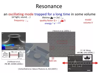
420 nm Resonance an oscillating mode trapped for a long time in some volume (of light, sound, …) frequency w0 lifetime t >> 2π/w0 quality factor Q = w0t/2 energy ~ e–w0t/Q modal volume V [ Notomi et al. (2005). ] [ C.-W. Wong, APL84, 1242 (2004). ] [ Schliesser et al., PRL 97, 243905 (2006) ] [ Eichenfield et al. Nature Photonics1, 416 (2007) ]
Why Resonance? an oscillating mode trapped for a long time in some volume • long time = narrow bandwidth … filters (WDM, etc.) — 1/Q = fractional bandwidth • resonant processes allow one to “impedance match” hard-to-couple inputs/outputs • long time, small V … enhanced wave/matter interaction — lasers, nonlinear optics, opto-mechanical coupling, sensors, LEDs, thermal sources, …
How Resonance? need mechanism to trap light for long time metallic cavities: good for microwave, dissipative for infrared [ Xu & Lipson (2005) ] 10µm VCSEL [fotonik.dtu.dk] ring/disc/sphere resonators: a waveguide bent in circle, bending loss ~ exp(–radius) [ llnl.gov ] [ Akahane, Nature425, 944 (2003) ] photonic bandgaps (complete or partial + index-guiding) (planar Si slab)
Understanding Resonant Systems • Option 1: Simulate the whole thing exactly — many powerful numerical tools — limited insight into a single system — can be difficult, especially for weak effects (nonlinearities, etc.) • Option 2: Solve each component separately, couple with explicit perturbative method (one kind of “coupled-mode” theory) [ Schliesser et al., PRL 97, 243905 (2006) ] • Option 3: abstract the geometry into its most generic form …write down the most general possible equations …constrain by fundamental laws (conservation of energy) …solve for universal behaviors of a whole class of devices … characterized via specific parameters from option 2
“Temporal coupled-mode theory” • Generic form developed by Haus, Louisell, & others in 1960s & early 1970s • Haus, Waves & Fields in Optoelectronics (1984) • Reviewed in our Photonic Crystals: Molding the Flow of Light, 2nd ed., ab-initio.mit.edu/book • Equations are generic reappear in many forms in many systems, rederived in many ways (e.g. Breit–Wigner scattering theory) • full generality is not always apparent (modern name coined by S. Fan @ Stanford)
420 nm TCMT example: a linear filter [ C.-W. Wong, APL84, 1242 (2004). ] [ Notomi et al. (2005). ] [ Takano et al. (2006) ] = abstractly: two single-mode i/o ports + one resonance port 1 port 2 resonant cavity frequency w0, lifetimet [ Ou & Kimble (1993) ]
can be relaxed Temporal Coupled-Mode Theoryfor a linear filter s1+ input a output s1– s2– resonant cavity frequency w0, lifetimet |s|2 = power |a|2 = energy assumes only: • exponential decay (strong confinement) • linearity • conservation of energy • time-reversal symmetry
Temporal Coupled-Mode Theoryfor a linear filter s1+ input a output s1– s2– resonant cavity frequency w0, lifetimet |s|2 = flux |a|2 = energy 1 T = Lorentzian filter transmission T = |s2–|2 / |s1+|2 w w0
Resonant Filter Example Lorentzian peak, as predicted. An apparent miracle: ~ 100% transmission at the resonant frequency cavity decays to input/output with equal rates At resonance, reflected wave destructively interferes with backwards-decay from cavity & the two exactly cancel.
Some interesting resonant transmission processes input power Resonant LED emission luminus.com output power ~ 40% eff. (narrow-band) resonant absorption in a thin-film photovoltaic Wireless resonant power transfer [ M. Soljacic, MIT (2007) ] witricity.com [ e.g. Ghebrebrhan (2009) ]
Wide-angle Splitters [ S. Fan et al., J. Opt. Soc. Am. B18, 162 (2001) ]
Waveguide Crossings [ S. G. Johnson et al., Opt. Lett.23, 1855 (1998) ]
Another interesting example: Channel-Drop Filters waveguide 1 Perfect channel-dropping if: Two resonant modes with: • even and odd symmetry • equal frequency (degenerate) • equal decay rates Coupler waveguide 2 (mirror plane) [ S. Fan et al., Phys. Rev. Lett. 80, 960 (1998) ]
FWHM …quality factor Q Dimensionless Losses: Q Q = w0t / 2 quality factor Q = # optical periods for energy to decay by exp(–2π) energy ~ exp(–w0t/Q) = exp(–2t/t) in frequency domain: 1/Q = bandwidth 1 T = Lorentzian filter from temporal coupled-mode theory: w w0
We want: Qr>> Qw 1 – transmission ~ 2Q /Qr Q = lifetime/period = frequency/bandwidth More than one Q… A simple model device (filters, bends, …): losses (radiation/absorption) TCMT worst case: high-Q (narrow-band) cavities
Nonlinearities + Microcavities? weak effects ∆n < 1% very intense fields & sensitive to small changes A simple idea: for the same input power, nonlinear effects are stronger in a microcavity That’s not all! nonlinearities + microcavities = qualitatively new phenomena
Nonlinear Optics Kerr nonlinearities c(3): (polarization ~ E3) • Self-Phase Modulation (SPM) = change in refractive index(w) ~ |E(w)|2 • Cross-Phase Modulation (XPM) = change in refractive index(w) ~ |E(w 2)|2 • Third-Harmonic Generation (THG) & down-conversion (FWM) = w3w, and back • etc… w w w’s 3w w w w Second-order nonlinearities c(2): (polarization ~ E2) • Second-Harmonic Generation (SHG) & down-conversion = w2w, and back • Difference-Frequency Generation (DFG) = w1, w2w1-w2 • etc…
Nonlinearities + Microcavities? weak effects ∆n < 1% very intense fields & sensitive to small changes A simple idea: for the same input power, nonlinear effects are stronger in a microcavity That’s not all! nonlinearities + microcavities = qualitatively new phenomena let’s start with a well-known example from 1970’s…
Linear response: Lorenzian Transmisson A Simple Linear Filter in out
Linear response: Lorenzian Transmisson shifted peak? + nonlinear index shift = w shift Filter + Kerr Nonlinearity? in out Kerr nonlinearity: ∆n ~ |E|2
stable unstable [ Soljacic et al., PRE Rapid. Comm.66, 055601 (2002). ] stable Power threshold ~ V/Q2 (in cavity with V ~ (l/2)3, for Si and telecom bandwidth power ~ mW) Optical Bistability [ Felber and Marburger., Appl. Phys. Lett.28, 731 (1978). ] Logic gates, switching, rectifiers, amplifiers, isolators, … Bistable (hysteresis) response (& even multistable for multimode cavity)
TCMT for Bistability [ Soljacic et al., PRE Rapid. Comm.66, 055601 (2002). ] input a output s1+ s2– resonant cavity frequency w0, lifetimet, SPM coefficienta ~ c(3) (from perturbation theory) |s|2 = power |a|2 = energy gives cubic equation for transmission … bistable curve
TCMT + Perturbation Theory SPM = small change in refractive index … evaluate ∆w by 1st-order perturbation theory • all relevant parameters (w, t or Q, a) can be computed from the resonant mode of the linear system
semi-analytical numerical Accuracy of Coupled-Mode Theory [ Soljacic et al., PRE Rapid. Comm.66, 055601 (2002). ]
[ Notomi et al. (2005). ] 420 nm Optical Bistability in Practice [ Xu & Lipson, 2005 ] 10µm Q ~ 30,000 V ~ 10 optimum Power threshold ~ 40 µW Q ~ 10,000 V ~ 300 optimum Power threshold ~ 10 mW
Experimental Bistable Switch [ Notomi et al., Opt. Express13 (7), 2678 (2005). ] Silicon-on-insulator 420 nm Q ~ 30,000 Power threshold ~ 40 µW Switching energy ~ 4 pJ