Matrix Realization and Controller Feedback System
Explore the controllability and observability of matrices to design a feedback controller in this realization study. Dive into matrix norms and rank computation.

Matrix Realization and Controller Feedback System
E N D
Presentation Transcript
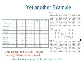
term ch2 ch3 ch4 ch5 ch6 ch7 ch8 ch9 controllability 1 1 0 0 1 0 0 1 observability 1 0 0 0 1 1 0 1 realization 1 0 1 0 1 0 1 0 feedback 0 1 0 0 0 1 0 0 controller 0 1 0 0 1 1 0 0 observer 0 1 1 0 1 1 0 0 transfer function 0 0 0 0 1 1 0 0 polynomial 0 0 0 0 1 0 1 0 matrices 0 0 0 0 1 0 1 1 Yet another Example U (9x7) = 0.3996 -0.1037 0.5606 -0.3717 -0.3919 -0.3482 0.1029 0.4180 -0.0641 0.4878 0.1566 0.5771 0.1981 -0.1094 0.3464 -0.4422 -0.3997 -0.5142 0.2787 0.0102 -0.2857 0.1888 0.4615 0.0049 -0.0279 -0.2087 0.4193 -0.6629 0.3602 0.3776 -0.0914 0.1596 -0.2045 -0.3701 -0.1023 0.4075 0.3622 -0.3657 -0.2684 -0.0174 0.2711 0.5676 0.2750 0.1667 -0.1303 0.4376 0.3844 -0.3066 0.1230 0.2259 -0.3096 -0.3579 0.3127 -0.2406 -0.3122 -0.2611 0.2958 -0.4232 0.0277 0.4305 -0.3800 0.5114 0.2010 S (7x7) = 3.9901 0 0 0 0 0 0 0 2.2813 0 0 0 0 0 0 0 1.6705 0 0 0 0 0 0 0 1.3522 0 0 0 0 0 0 0 1.1818 0 0 0 0 0 0 0 0.6623 0 0 0 0 0 0 0 0.6487 V (7x8) = 0.2917 -0.2674 0.3883 -0.5393 0.3926 -0.2112 -0.4505 0.3399 0.4811 0.0649 -0.3760 -0.6959 -0.0421 -0.1462 0.1889 -0.0351 -0.4582 -0.5788 0.2211 0.4247 0.4346 -0.0000 -0.0000 -0.0000 -0.0000 0.0000 -0.0000 0.0000 0.6838 -0.1913 -0.1609 0.2535 0.0050 -0.5229 0.3636 0.4134 0.5716 -0.0566 0.3383 0.4493 0.3198 -0.2839 0.2176 -0.5151 -0.4369 0.1694 -0.2893 0.3161 -0.5330 0.2791 -0.2591 0.6442 0.1593 -0.1648 0.5455 0.2998 T This happens to be a rank-7 matrix -so only 7 dimensions required Singular values = Sqrt of Eigen values of AAT
Formally, this will be the rank-k (2) matrix that is closest to M in the matrix norm sense U (9x7) = 0.3996 -0.1037 0.5606 -0.3717 -0.3919 -0.3482 0.1029 0.4180 -0.0641 0.4878 0.1566 0.5771 0.1981 -0.1094 0.3464 -0.4422 -0.3997 -0.5142 0.2787 0.0102 -0.2857 0.1888 0.4615 0.0049 -0.0279 -0.2087 0.4193 -0.6629 0.3602 0.3776 -0.0914 0.1596 -0.2045 -0.3701 -0.1023 0.4075 0.3622 -0.3657 -0.2684 -0.0174 0.2711 0.5676 0.2750 0.1667 -0.1303 0.4376 0.3844 -0.3066 0.1230 0.2259 -0.3096 -0.3579 0.3127 -0.2406 -0.3122 -0.2611 0.2958 -0.4232 0.0277 0.4305 -0.3800 0.5114 0.2010 S (7x7) = 3.9901 0 0 0 0 0 0 0 2.2813 0 0 0 0 0 0 0 1.6705 0 0 0 0 0 0 0 1.3522 0 0 0 0 0 0 0 1.1818 0 0 0 0 0 0 0 0.6623 0 0 0 0 0 0 0 0.6487 V (7x8) = 0.2917 -0.2674 0.3883 -0.5393 0.3926 -0.2112 -0.4505 0.3399 0.4811 0.0649 -0.3760 -0.6959 -0.0421 -0.1462 0.1889 -0.0351 -0.4582 -0.5788 0.2211 0.4247 0.4346 -0.0000 -0.0000 -0.0000 -0.0000 0.0000 -0.0000 0.0000 0.6838 -0.1913 -0.1609 0.2535 0.0050 -0.5229 0.3636 0.4134 0.5716 -0.0566 0.3383 0.4493 0.3198 -0.2839 0.2176 -0.5151 -0.4369 0.1694 -0.2893 0.3161 -0.5330 0.2791 -0.2591 0.6442 0.1593 -0.1648 0.5455 0.2998 U2 (9x2) = 0.3996 -0.1037 0.4180 -0.0641 0.3464 -0.4422 0.1888 0.4615 0.3602 0.3776 0.4075 0.3622 0.2750 0.1667 0.2259 -0.3096 0.2958 -0.4232 S2 (2x2) = 3.9901 0 0 2.2813 V2 (8x2) = 0.2917 -0.2674 0.3399 0.4811 0.1889 -0.0351 -0.0000 -0.0000 0.6838 -0.1913 0.4134 0.5716 0.2176 -0.5151 0.2791 -0.2591 T U2*S2*V2 will be a 9x8 matrix That approximates original matrix
Coordinate transformation inherent in LSI Doc rep T-D = T-F*F-F*(D-F)T Mapping of keywords into LSI space is given by T-F*F-F Mapping of a doc d=[w1….wk] into LSI space is given by d’*T-F*(F-F)-1 For k=2, the mapping is: The base-keywords of The doc are first mapped To LSI keywords and Then differentially weighted By S-1 LSx LSy controllability observability realization feedback controller observer Transfer function polynomial matrices 1.5944439 -0.2365708 1.6678618 -0.14623132 1.3821706 -1.0087909 0.7533309 1.05282 1.4372339 0.86141896 1.6259657 0.82628685 1.0972775 0.38029274 0.90136355 -0.7062905 1.1802715 -0.96544623 LSIy ch3 controller LSIx controllability
Querying T-F To query for feedback controller, the query vector would be q = [0 0 0 1 1 0 0 0 0]' (' indicates transpose), since feedback and controller are the 4-th and 5-th terms in the index, and no other terms are selected. Let q be the query vector. Then the document-space vector corresponding to q is given by: q'*TF(2)*inv(FF(2) ) = Dq For the feedback controller query vector, the result is: Dq = 0.1376 0.3678 To find the best document match, we compare the Dq vector against all the document vectors in the 2-dimensional V2 space. The document vector that is nearest in direction to Dq is the best match. The cosine values for the eight document vectors and the query vector are: -0.3747 0.9671 0.1735 -0.9413 0.0851 0.9642 -0.7265 -0.3805 F-F D-F Centroid of the terms In the query (with scaling) -0.37 0.967 0.173 -0.94 0.08 0.96 -0.72 -0.38
DB-Regression example Started with D-T matrix Used the term axes as T-F; and the doc rep as D-F*F-F Q is converted into q’*T-F Chapter/Medline etc examples Started with T-D matrix Used term axes as T-F*FF and doc rep as D-F Q is converted to q’*T-F*FF-1 Variations in the examples We will stick to this convention
Query Expansion Add terms that are closely related to the query terms to improve precision and recall. Two variants: Local only analyze the closeness among the set of documents that are returned Global Consider all the documents in the corpus a priori How to decide closely related terms? THESAURI!! -- Hand-coded thesauri (Roget and his brothers) -- Automatically generated thesauri --Correlation based (association, nearness) --Similarity based (terms as vectors in doc space)
Co-occurrence analysis: Terms that are related to terms in the original query may be added to the query. Two terms are related if they have high co-occurrence in documents. Let n be the number of documents; n1 and n2 be # documents containing terms t1 and t2, m be the # documents having both t1 and t2 If t1 and t2 are independent If t1 and t2 are correlated Correlation/Co-occurrence analysis >> if Inversely correlated Measure degree of correlation
Let Mij be the term-document matrix For the full corpus (Global) For the docs in the set of initial results (local) (also sometimes, stems are used instead of terms) Correlation matrix C = MMT (term-doc Xdoc-term = term-term) Association Clusters Un-normalized Association Matrix Normalized Association Matrix Nth-Association Cluster for a term tu is the set of terms tv such that Suv are the n largest values among Su1, Su2,….Suk
Example 11 4 6 4 34 11 6 11 26 Correlation Matrix d1d2d3d4d5d6d7 K1 2 1 0 2 1 1 0 K2 0 0 1 0 2 2 5 K3 1 0 3 0 4 0 0 Normalized Correlation Matrix 1.0 0.097 0.193 0.097 1.0 0.224 0.193 0.224 1.0 1thAssoc Cluster for K2is K3
Scalar clusters Even if terms u and v have low correlations, they may be transitively correlated (e.g. a term w has high correlation with u and v). Consider the normalized association matrix S The “association vector” of term u Au is (Su1,Su2…Suk) To measure neighborhood-induced correlation between terms: Take the cosine-theta between the association vectors of terms u and v Nth-scalar Cluster for a term tu is the set of terms tv such that Suv are the n largest values among Su1, Su2,….Suk
Example Normalized Correlation Matrix AK1 USER(43): (neighborhood normatrix) 0: (COSINE-METRIC (1.0 0.09756097 0.19354838) (1.0 0.09756097 0.19354838)) 0: returned 1.0 0: (COSINE-METRIC (1.0 0.09756097 0.19354838) (0.09756097 1.0 0.2244898)) 0: returned 0.22647195 0: (COSINE-METRIC (1.0 0.09756097 0.19354838) (0.19354838 0.2244898 1.0)) 0: returned 0.38323623 0: (COSINE-METRIC (0.09756097 1.0 0.2244898) (1.0 0.09756097 0.19354838)) 0: returned 0.22647195 0: (COSINE-METRIC (0.09756097 1.0 0.2244898) (0.09756097 1.0 0.2244898)) 0: returned 1.0 0: (COSINE-METRIC (0.09756097 1.0 0.2244898) (0.19354838 0.2244898 1.0)) 0: returned 0.43570948 0: (COSINE-METRIC (0.19354838 0.2244898 1.0) (1.0 0.09756097 0.19354838)) 0: returned 0.38323623 0: (COSINE-METRIC (0.19354838 0.2244898 1.0) (0.09756097 1.0 0.2244898)) 0: returned 0.43570948 0: (COSINE-METRIC (0.19354838 0.2244898 1.0) (0.19354838 0.2244898 1.0)) 0: returned 1.0 Scalar (neighborhood) Cluster Matrix 1.0 0.226 0.383 0.226 1.0 0.435 0.383 0.435 1.0 1thScalar Cluster for K2is still K3
Querying To query for database index, the query vector would be q = [1 0 1 0 0 0 ] since database and index are the 1st and 3rd terms in the index, and no other terms are selected. Let q be the query vector. Then the document-space vector corresponding to q is given by: q'*U2*inv(S2) = Dq To find the best document match, we compare the Dq vector against all the document vectors in the 2-dimensional doc space. The document vector that is nearest in direction to Dq is the best match. The cosine values for the eight document vectors and the query vector are: -0.3747 0.9671 0.1735 -0.9413 0.0851 0.9642 -0.7265 -0.3805 Centroid of the terms In the query (with scaling)