Download
1 / 14
140 likes | 265 Vues
This paper explores the integration of systematic network coding in full-duplex relay systems, addressing complexities in packet transmission and decoding. It introduces a relay model utilizing both systematic and random linear network coding (RLNC), assessing the trade-offs between decoding complexity and network performance. Through a Markov chain model, the authors analyze transition probabilities, mean completion times, and the impact of uncoded packet transmission. The findings highlight a balance between performance gains and decoding complexity, paving the way for future studies in multi-hop systems.

E N D
Systematic Network Codingwith the aid of a Full-Duplex Relay June 12, ICC GiulianoGiacaglia, Xiaomeng Shi, MinJiKim, Daniel Lucani, Muriel Médard
Relay Introduction P2 P3 Sender Receiver P1 • Packet-erasure relay channel • Different frequency assigned for transmission from sender and relay • Relay can transmit and receive simultaneously Applications: • Cellular network using relays • Cooperative schemes using multiple interfaces Conventional network coding solution (throughput optimal) • Systematic network coding @sender • Random linear network coding (RLNC) @relay • Issue: large decoding complexity @ receiverwith high packet loss rate P1. What is the complexity-performance trade off of a systematic relay? • Suboptimal solution from delay perspective • Increases expected number of uncoded packets received
System Assumptions Assumptions: • Sender broadcasts M packets • Slotted transmissions • Duplex relay Solution: Two stage transmission • Systematic stage: Systematic relay: forwards uncodedpkts, no recoding RLNC relay: performs RLNC using all uncodedpktsin memory • RLNC Stage: • Sender: broadcasts RLNC pkts • Relay: performs RLNC on all pkts (coded or uncoded) in memory Transmission terminates when receiver ACKs M dofsreceived
System Model Markov chain model • State of the network: (i, j, k) • i= # dof @ receiver • j= # dof @ relay • k = # dofs shared by receiver and relay • (i,j,k) valid if i+j-k ≤ M, i ≤ M, j ≤ M, 0 ≤ k ≤ min(i, j) • Transmission initiates at (0,0,0) and terminates at (M, j, k) p2 0 1 2 1 2 0 0 2 p1 p1 + p2 p1 p1 + p2 p1 + p2 p2 p1 + p2 p1 p2
State Transition Probabilities Transition probabilities for non-systematic case • Combinatorial approach • Two major scenarios • i+j-k = M Relay and receiver have jointly all dof • i+j-k < M Relay and receiver do not have jointly all dof • Useful also for second stage of systematic relay Case 4P1(1-P2)P3 Case 3(1-P1)(1-P2)(1-P3) Case 1P1(1-P2)(1-P3) Case 2(1-P1)(1-P2)P3 Case 8P1P2P3 Case 7(1-P1)P2(1-P3) Case 5(1-P1)P2P3 Case 6P1P2 (1-P3)
Performance Analysis and Metrics Transition probabilities for systematic relay • Transition probabilities and evolution is different in the systematic stage • In RLNC stage, same as the non-systematic relay case Metrics • Mean completion time • Expected # uncoded packets received via the systematic relay • Expected # of additional coded packets via the systematic relay • Decoding complexity @ Receiver on the order of
Numerical Results P3 P2 • Delay gap < 1dB P1 • Additional number of uncoded packets grows with P1
Numerical Results P3 P2 • Delay gap < 1dB P1 • The additional number of uncoded packets decreases with P3
Conclusion • Studied the trade-off between performance and complexity • Simple solution @ relay • Used number of uncoded packets as proxy to decoding complexity • Price of complexity is reduced with small cost in delay (<1dB) • Provided analysis to characterize the system • Markov model • Transition prob required combinatorial approach • Captures dependence between relay and receiver knowledge (critical) • Future work: multi-hop • Analysis may be hard • Local optimization heuristics • Half-duplex constraints • Judicious feedback use
System Model: Systematic Relay • Stage One: • Q(0,0,0)→ (i,j,k) = Prob of being in state (i,j,k) at the end of Stage One. • Result of three independent Bernoulli Trials • Stage Two: Same system evolution as the non-systematic case • Expected # uncoded packets received via the systematic relay • Decoding complexity @ Receiver on the order of O((M-U)3) + O(U(M-U))
Decoding Complexity and Delay P3 P2 Normalized # uncodedpackets received via the systematic relay P1 Normalized Mean Completion Time T/M
Relay Relay Non-System vs. Systematic Relay • Non-systematic: always transmit linear combination of ALL received pkts. Sender Sender Receiver Receiver loss • Systematic: forwards any received uncodedpackets loss
System Model • State of the network: (i, j, k) • i= # dof @ Receiver • j= # dof @ Relay • k = # dofs shared by Receiver and Relay • (i,j,k) valid if i+j-k ≤ M, i ≤ M, j ≤ M, 0 ≤ k ≤ min(i, j) • Transmission initiates at (0,0,0) • Transmission terminates at (M, j, k) • P(i,j,k)→ (i’,j’,k’) = Prob of transiting from state (i,j,k) to state (i’,j’,k’) • Expected time to reach a terminating state from (i,j,k): • Expected completion time: