Grid-based Map Analysis (Spatial Analysis/Statistics)
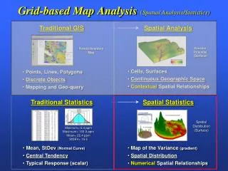
Traditional GIS. Spatial Analysis. Forest Inventory Map. Erosion Potential (Surface). Points, Lines, Polygons Discrete Objects Mapping and Geo-query. Cells, Surfaces Continuous Geographic Space Contextual Spatial Relationships. Spatial Statistics. Traditional Statistics.

Grid-based Map Analysis (Spatial Analysis/Statistics)
E N D
Presentation Transcript
Traditional GIS Spatial Analysis Forest Inventory Map Erosion Potential (Surface) • Points, Lines, Polygons • Discrete Objects • Mapping and Geo-query • Cells, Surfaces • Continuous Geographic Space • Contextual Spatial Relationships Spatial Statistics Traditional Statistics Spatial Distribution (Surface) Minimum= 5.4 ppm Maximum= 103.0 ppm Mean= 22.4 ppm StDEV= 15.5 • Mean, StDev (Normal Curve) • Central Tendency • Typical Response (scalar) • Map of the Variance (gradient) • Spatial Distribution • Numerical Spatial Relationships Grid-based Map Analysis (Spatial Analysis/Statistics)
Spatial Statistics • Surface modelingmaps the “spatial distribution” and pattern of point data… • Map Generalization— characterizes spatial trends (e.g., titled plane) • Spatial Interpolation— deriving spatial distributions (e.g., IDW, Krig) • Other— roving window/facets (e.g., density surface; tessellation) • Data Mininginvestigates the “numerical” relationships in mapped data… • Descriptive— aggregate statistics (e.g., average/stdev, similarity, clustering) • Predictive— relationships among maps (e.g., regression) • Prescriptive— appropriate actions (e.g., optimization) Grid-Based Map Analysis • Spatial analysisinvestigates the “contextual” relationships in mapped data… • Reclassify— reassigning map values (position; value; size, shape; contiguity) • Overlay— map overlay (point-by-point; region-wide; map-wide) • Distance— proximity and connectivity (movement; optimal paths; visibility) • Neighbors— ”roving windows” (slope/aspect; diversity; anomaly) (Berry)
Point Density analysis identifies the number of customers with a specified distance of each grid location Point Density Analysis Roving Window (count) (Berry)
Pockets of unusually high customer density are identified as more than one standard deviation above the mean Identifying Unusually High Density (Berry)
Surface Modeling(Density Surface) Roving Window Total number of counts within 6-cell radius Hugag Density Surface Hugag Counts Avg- 17.5 StDev= 15.0 Discrete Map Surface 2 Hugags every 30 min for 30 days Hugag Activity draped over Elevation Hugag Density Surface Modeling “Counts” the number of occurrences within a specified “roving window” reach— higher values indicate concentrations of occurrence …from discrete observations to continuous spatial distribution Continuous Map Surface Most of the activity is in the NE (Short Exercise #6) (Berry)
Spatial Interpolation(Smoothing the Variability) The “iterative smoothing” process is similar to slapping a big chunk of modeler’s clay over the “data spikes,” then taking a knife and cutting away the excess to leave a continuous surface that encapsulates the peaks and valleys implied in the original field samples …repeated smoothing slowly “erodes” the data surface to a flat plane= AVERAGE (digital slide show SSTAT2) (Berry)
Inverse Distance Weighted Approach Tobler’s First Law of Geography— nearby things are more alike than distant things 1/DPower (Berry)
Spatial Autocorrelation (Kriging) Tobler’s First Law of Geography— nearby things are more alike than distant things Variogram— plot of sample data similarity as a function of distance between samples …Kriging uses regional variable theory based on an underlying variogram to develop custom weights based on trends in the sample data (proximity and direction) …uses Variogram Equation instead of a fixed 1/DPower Geometric Equation (Berry)
Spatial Interpolation Geometric facets Thiessen Polygons Map Generalization Surface Modeling Methods (Surfer) Inverse Distance to a Power— weighted average of samples in the summary window such that the influence of a sample point declines with “simple” distance Modified Shepard’s Method— uses an inverse distance “least squares” method that reduces the “bull’s-eye” effect around sample points Radial Basis Function— uses non-linear functions of “simple” distance to determine summary weights Kriging— summary of samples based on distance and angular trends in the data Natural Neighbor—weighted average of neighboring samples where the weights are proportional to the “borrowed area” from the surrounding points (based on differences in Thiessen polygon sets) Minimum Curvature— analogous to fitting a thin, elastic plate through each sample point using a minimum amount of bending (Spatial Interpolation) Nearest Neighbor— assigns the value of the nearest sample point Triangulation— identifies the “optimal” set of triangles connecting all of the sample points (Geometric Facets) Polynomial Regression— fits an equation to the entire set of sample points (Map Generalization) (Berry)
Spatial Interpolation is similar to throwing a blanket over the “data spikes” to conforming to the geographic pattern of the data. Spatial Interpolation …all interpolation algorithms assume that… 1) “nearby things are more alike than distant things” (spatial autocorrelation), 2) appropriate sampling intensity (ample number of samples), and a 3) suitable sampling pattern …the interpolated surfaces “map the spatial variation” in the data samples (Berry)
Comparison of the IDW interpolated surface to the whole field average shows LARGE differences in localized estimates Comparison of the IDW and Krig interpolated surfaces shows small differences in in localized estimates Comparing Spatial Interpolation Results (Berry)
Spatial Interpolation Use Surfer to interpolate a continuous surface… …and generate contour and solid surface plots Density Surface Derivation (Use MapCalc to derive a customer density surface) • SCAN Total_Customers TOTAL WITHIN 6 FOR Customer_density6 • RENUMBER Customer_density6 ASSIGNING 0 TO 0 THRU 33.7 ASSIGNING 1 TO 33.7 THRU 1000 FOR Customer_highDensity Use MapCalc to create a density surface (total count) Surface Modeling (Full Exercise #6) (Berry)
Spatial Interpolation techniques use “roving windows” to summarize sample values within a specified reach of each map location. Window shape/size and summary technique result in different interpolation surfaces for a given set of field data …no single techniques is best for all data. AVG= 23 everywhere Inverse Distance Weighted (IDW) technique weights the samples such that values farther away contribute less to the average …1/Distance Power Spatial Interpolation Techniques Characterizes the spatial distribution by fitting a mathematical equation to localized portions of the data (roving window) (Berry)
Assessing Interpolation Results (Residual Analysis) …the best map is the one that has the “best guesses” AVG= 23 Spatial Interpolation(Evaluating performance) (Berry)
A Map of Error (Residual Map) …shows you where your estimates are likely good/bad Spatial Interpolation (Spatially characterizing error) (Berry)
Basis for… Surface Modeling …understanding relationships within a single map layer Basis for… Spatial Data Mining …understanding relationships among map layers Spatial Dependency (Spatial Autocorrelation & Correlation) Spatial Variable Dependence— what occurs at a location in geographic space is related to: • the conditions of that variable at nearby locations, termed Spatial Autocorrelation(intra-variable dependence for Surface Modeling) • the conditions of other variables at • that location, termed Spatial Correlation • (inter-variable dependence for Spatial Data Mining) (Berry)
Spatial analysisinvestigates the “contextual” relationships in mapped data… • Reclassify— reassigning map values (position; value; size, shape; contiguity) • Overlay— map overlay (point-by-point; region-wide; map-wide) • Distance— proximity and connectivity (movement; optimal paths; visibility) • Neighbors— ”roving windows” (slope/aspect; diversity; anomaly) Spatial Statistics • Surface modelingmaps the “spatial distribution” and pattern of point data… • Map Generalization— characterizes spatial trends (e.g., titled plane) • Spatial Interpolation— deriving spatial distributions (e.g., IDW, Krig) • Other— roving window/facets (e.g., density surface; tessellation) Grid-Based Map Analysis • Data Mininginvestigates the “numerical” relationships in mapped data… • Descriptive— aggregate statistics (e.g., average/stdev, similarity, clustering) • Predictive— relationships among maps (e.g., regression) • Prescriptive— appropriate actions (e.g., optimization) (Berry)
Interpolated Spatial Distribution Phosphorous (P) Visualizing Spatial Relationships What spatial relationships do you see? …do relatively high levels of P often occur with high levels of K and N? …how often? …where? (Berry)
Identifying Unusually High Measurements …isolate areas with mean + 1 StDev (tail of normal curve) (Berry)
Level Slicing …simply multiply the two maps to identify joint coincidence 1*1=1 coincidence (any 0 results in zero) (Berry)
Multivariate Data Space …sum of a binary progression (1, 2 ,4 8, 16, etc.) provides level slice solutions for many map layers (Berry)
Calculating Data Distance …an n-dimensional plot depicts the multivariate distribution— the distance between points determines the relative similarity in data patterns …the closest floating ball is the least similar (largest data distance) from the comparison point (Berry)
Identifying Map Similarity …the relative data distance between the comparison point’s data pattern and those of all other map locations form a Similarity Index …the green tones indicate field locations with fairly similar P, K and N levels; red tones indicate dissimilar areas (Berry)
…a map stack is a spatially organized set of numbers …groups of “floating balls” in data space identify locations in the field with similar data patterns– data zones (Cyber-Farmer, Circa 1990) …fertilization rates vary for the different clusters “on-the-fly” Variable Rate Application Clustering Maps for Data Zones (Berry)
Evaluating Clustering Results …graphical and statistics procedures assess how “distinct” clusters are— Clustering Performance …distinct in K and N (less), but not distinct in P (Berry)
Similarity Map Cluster Map (Short Exercise #7) Regional Average Composite Descriptive Prescriptive Scatter Plot Univariate Regression Multivariate Regression Spatial Data Mining (Full Exercise #7) • Spatial statistics … use MapCalcto implement derive relationships among P, K, N and Yield in a farmer’s field (Berry)
The Precision Ag Process(Fertility example) Steps 1) – 3) On-the-Fly Yield Map Map Analysis Step 4) Cyber-Farmer, Circa 1992 Farm dB Zone 3 Zone 2 Zone 1 Variable Rate Application Prescription Map Step 6) Step 5) As a combine moves through a field it 1) uses GPS to check its location then 2) checks the yield at that location to 3) create a continuous map of the yield variation every few feet. This map is 4) combined with soil, terrain and other maps to derive 5) a “Prescription Map” that is used to 6) adjust fertilization levels every few feet in the field (variable rate application). (Berry)
Mapped data that exhibits high spatial dependency create strong prediction functions. As in traditional statistical analysis, spatial relationships can be used to predict outcomes… …the difference is that spatial statistics predicts where responses will be high or low Spatial Data Mining Precision Farming is just one example of applying spatial statistics and data mining techniques Geo-business SDM (Berry)
Data Analysis Perspectives(Review) Traditional Analysis Map Analysis (Data Space — Non-spatial Statistics) (Geographic Space — Spatial Statistics) Field Data Standard Normal Curve fit to the data Spatially Interpolated data Central Tendency Average = 22.0 StDev = 18.7 Typical How Typical Discrete Spatial Object (Generalized) Continuous Spatial Distribution (Detailed) 22.0 28.2 Identifies the Central Tendency Maps the Variance (Berry)
Spatial Analysis Spatial Statistics Grid-Based Map Analysis (Review) • Spatial Analysisinvestigates the “contextual” relationships in mapped data… • Reclassify— reassigning map values (position; value; size, shape; contiguity) • Overlay— map overlay (point-by-point; region-wide; map-wide) • Distance— proximity and connectivity (movement; optimal paths; visibility) • Neighbors— ”roving windows” (slope/aspect; diversity; anomaly) • Surface Modelingmaps the “spatial distribution” and pattern of point data… • Map Generalization— characterizes spatial trends (e.g., titled plane) • Spatial Interpolation— deriving spatial distribution (e.g., IDW, Krig) • Other— roving window (e.g., density surface; tessellation) • Data Mininginvestigates the “numerical” relationships in mapped data… • Descriptive— aggregate statistics (e.g., average/stdev, similarity) • Predictive— relationships among maps (e.g., regression) • Prescriptive— appropriate actions (e.g., optimization) (Berry)
Tutorial Exercises Workshop Exercises MapCalc Tutorial Short & Full Exercise Sets Workshop CD Surfer Tutorial See Default.htm Complete Experience NEW BOOK — seethe description of the Map Analysisbook (Berry, 2007; GeoTec Media)at…www.innovativegis.com/basis …develops a structured view of the important concepts, considerations and procedures involved in grid-based map analysis. …the companion CD contains further readings and software for hands-on experience with the material presented. More Map Analysis Experience(MapCalc & Surfer) (Berry)
…but before we leave Spatial Statistics (Surface Modeling and Spatial Data Mining—descriptive, predictive and prescriptive) to tackle GIS Modeling, any… Questions? Questions? (Berry)